Triangular Meshes and Basic Plotting#
%matplotlib inline
import matplotlib.pylab as plt
anatomy of a triangular mesh#
Triangular meshes are often represented as a collection of corner points (vertices) and a collection of triangles. Triangles are typically represented as three indices from within the vertex arrays.
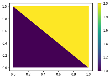
Let’s create four vertices at the corner of the unit square and fill the area with two triangles. Each of the two triangles will cary a value (think of surface temperature, some fluxes etc…).
xs = [0, 1, 0, 1]
ys = [0, 0, 1, 1]
tris = [[0, 1, 2], [1, 2, 3]]
values = [1, 2]
Matplotlib’s tripcolor takes all of these pieces and creates a plot out of it.
plt.tripcolor(xs, ys, tris, values)
plt.colorbar()
<matplotlib.colorbar.Colorbar at 0x2b8079edc790>
application to model data#
Let’s fetch some data from the intake catalog, attach the gridfile to it and select a lat-lon region for plotting.
import intake
import numpy as np
import xarray as xr
import yaml
from gridlocator import (
    merge_grid,
)  # gridlocator.py can be found further below at 'playing with triangles'
col_url = "/pf/k/k202134/DYAMOND/Processing/full_catalog.json"
col = intake.open_esm_datastore(col_url)
res = col.search(
    variable="prw",
    project="NextGEMS",
    model="ICON-SAP-5km",
    ensemble_member="dpp0052",
    operation="inst",
)
# res
d = res.to_dataset_dict(cdf_kwargs={"chunks": {"time": 1}})
--> The keys in the returned dictionary of datasets are constructed as follows:
	'project.institute.model.experiment.domain.frequency.grid.level_type.ensemble_member.operation'
ds = merge_grid(next(iter(d.values())))
ds
<xarray.Dataset>
Dimensions:                         (time: 1969, cell: 20971520, nv: 3, vertex: 10485762, ne: 6, edge: 31457280, no: 4, nc: 2, max_stored_decompositions: 4, two_grf: 2, cell_grf: 14, max_chdom: 1, edge_grf: 24, vert_grf: 13)
Coordinates:
  * time                            (time) float64 2.02e+07 ... 2.02e+07
    clon                            (cell) float64 ...
    clat                            (cell) float64 ...
    vlon                            (vertex) float64 ...
    vlat                            (vertex) float64 ...
    elon                            (edge) float64 ...
    elat                            (edge) float64 ...
Dimensions without coordinates: cell, nv, vertex, ne, edge, no, nc, max_stored_decompositions, two_grf, cell_grf, max_chdom, edge_grf, vert_grf
Data variables: (12/92)
    prw                             (time, cell) float32 dask.array<chunksize=(1, 20971520), meta=np.ndarray>
    clon_vertices                   (cell, nv) float64 ...
    clat_vertices                   (cell, nv) float64 ...
    vlon_vertices                   (vertex, ne) float64 ...
    vlat_vertices                   (vertex, ne) float64 ...
    elon_vertices                   (edge, no) float64 ...
    ...                              ...
    edge_dual_normal_cartesian_x    (edge) float64 ...
    edge_dual_normal_cartesian_y    (edge) float64 ...
    edge_dual_normal_cartesian_z    (edge) float64 ...
    cell_circumcenter_cartesian_x   (cell) float64 ...
    cell_circumcenter_cartesian_y   (cell) float64 ...
    cell_circumcenter_cartesian_z   (cell) float64 ...
Attributes:
    uuidOfHGrid:             0f1e7d66-637e-11e8-913b-51232bb4d8f9
    references:              see MPIM/DWD publications
    history:                 /work/mh0287/k203123/GIT/icon-aes-dyw3/bin/icon ...
    intake_esm_varname:      ['prw']
    source:                  git@gitlab.dkrz.de:icon/icon-aes.git@83f3dcef81e...
    title:                   ICON simulation
    institution:             Max Planck Institute for Meteorology/Deutscher W...
    grid_file_uri:           http://icon-downloads.mpimet.mpg.de/grids/public...
    number_of_grid_used:     15
    CDI:                     Climate Data Interface version 1.8.3rc (http://m...
    Conventions:             CF-1.6
intake_esm_dataset_key: NextGEMS.MPIM-DWD-DKRZ.ICON-SAP-5km.Cycle1.atm.3...- time: 1969
- cell: 20971520
- nv: 3
- vertex: 10485762
- ne: 6
- edge: 31457280
- no: 4
- nc: 2
- max_stored_decompositions: 4
- two_grf: 2
- cell_grf: 14
- max_chdom: 1
- edge_grf: 24
- vert_grf: 13
- time(time)float642.02e+07 2.02e+07 ... 2.02e+07
- standard_name :
- time
- units :
- day as %Y%m%d.%f
- calendar :
- proleptic_gregorian
- axis :
- T
array([20200120. , 20200120.020833, 20200120.041667, ..., 20200229.958333, 20200229.979167, 20200301. ]) - clon(cell)float64...
- long_name :
- center longitude
- units :
- radian
- standard_name :
- grid_longitude
- bounds :
- clon_vertices
[20971520 values with dtype=float64]
- clat(cell)float64...
- long_name :
- center latitude
- units :
- radian
- standard_name :
- grid_latitude
- bounds :
- clat_vertices
[20971520 values with dtype=float64]
- vlon(vertex)float64...
- long_name :
- vertex longitude
- units :
- radian
- standard_name :
- grid_longitude
- bounds :
- vlon_vertices
[10485762 values with dtype=float64]
- vlat(vertex)float64...
- long_name :
- vertex latitude
- units :
- radian
- standard_name :
- grid_latitude
- bounds :
- vlat_vertices
[10485762 values with dtype=float64]
- elon(edge)float64...
- long_name :
- edge midpoint longitude
- units :
- radian
- standard_name :
- grid_longitude
- bounds :
- elon_vertices
[31457280 values with dtype=float64]
- elat(edge)float64...
- long_name :
- edge midpoint latitude
- units :
- radian
- standard_name :
- grid_latitude
- bounds :
- elat_vertices
[31457280 values with dtype=float64]
- prw(time, cell)float32dask.array<chunksize=(1, 20971520), meta=np.ndarray>
- standard_name :
- total_vapour
- long_name :
- vertically integrated water vapour
- units :
- kg m-2
- param :
- 64.1.0
- CDI_grid_type :
- unstructured
- number_of_grid_in_reference :
- 1
- level_type :
- atmosphere
Array Chunk Bytes 165.17 GB 83.89 MB Shape (1969, 20971520) (1, 20971520) Count 3980 Tasks 1969 Chunks Type float32 numpy.ndarray - clon_vertices(cell, nv)float64...
- units :
- radian
[62914560 values with dtype=float64]
- clat_vertices(cell, nv)float64...
- units :
- radian
[62914560 values with dtype=float64]
- vlon_vertices(vertex, ne)float64...
- units :
- radian
[62914572 values with dtype=float64]
- vlat_vertices(vertex, ne)float64...
- units :
- radian
[62914572 values with dtype=float64]
- elon_vertices(edge, no)float64...
- units :
- radian
[125829120 values with dtype=float64]
- elat_vertices(edge, no)float64...
- units :
- radian
[125829120 values with dtype=float64]
- ifs2icon_cell_grid(cell)float64...
- long_name :
- ifs to icon cells
[20971520 values with dtype=float64]
- ifs2icon_edge_grid(edge)float64...
- long_name :
- ifs to icon edge
[31457280 values with dtype=float64]
- ifs2icon_vertex_grid(vertex)float64...
- long_name :
- ifs to icon vertex
[10485762 values with dtype=float64]
- cell_area(cell)float64...
- long_name :
- area of grid cell
- units :
- m2
- standard_name :
- area
- grid_type :
- unstructured
- number_of_grid_in_reference :
- 1
[20971520 values with dtype=float64]
- dual_area(vertex)float64...
- long_name :
- areas of dual hexagonal/pentagonal cells
- units :
- m2
- standard_name :
- area
[10485762 values with dtype=float64]
- phys_cell_id(cell)int32...
- long_name :
- physical domain ID of cell
- grid_type :
- unstructured
- number_of_grid_in_reference :
- 1
[20971520 values with dtype=int32]
- phys_edge_id(edge)int32...
- long_name :
- physical domain ID of edge
[31457280 values with dtype=int32]
- lon_cell_centre(cell)float64...
- long_name :
- longitude of cell centre
- units :
- radian
- grid_type :
- unstructured
- number_of_grid_in_reference :
- 1
[20971520 values with dtype=float64]
- lat_cell_centre(cell)float64...
- long_name :
- latitude of cell centre
- units :
- radian
- grid_type :
- unstructured
- number_of_grid_in_reference :
- 1
[20971520 values with dtype=float64]
- lat_cell_barycenter(cell)float64...
- long_name :
- latitude of cell barycenter
- units :
- radian
- grid_type :
- unstructured
- number_of_grid_in_reference :
- 1
[20971520 values with dtype=float64]
- lon_cell_barycenter(cell)float64...
- long_name :
- longitude of cell barycenter
- units :
- radian
- grid_type :
- unstructured
- number_of_grid_in_reference :
- 1
[20971520 values with dtype=float64]
- longitude_vertices(vertex)float64...
- long_name :
- longitude of vertices
- units :
- radian
[10485762 values with dtype=float64]
- latitude_vertices(vertex)float64...
- long_name :
- latitude of vertices
- units :
- radian
[10485762 values with dtype=float64]
- lon_edge_centre(edge)float64...
- long_name :
- longitudes of edge midpoints
- units :
- radian
[31457280 values with dtype=float64]
- lat_edge_centre(edge)float64...
- long_name :
- latitudes of edge midpoints
- units :
- radian
[31457280 values with dtype=float64]
- edge_of_cell(nv, cell)int32...
- long_name :
- edges of each cellvertices
[62914560 values with dtype=int32]
- vertex_of_cell(nv, cell)int32...
- long_name :
- vertices of each cellcells ad
[62914560 values with dtype=int32]
- adjacent_cell_of_edge(nc, edge)int32...
- long_name :
- cells adjacent to each edge
[62914560 values with dtype=int32]
- edge_vertices(nc, edge)int32...
- long_name :
- vertices at the end of of each edge
[62914560 values with dtype=int32]
- cells_of_vertex(ne, vertex)int32...
- long_name :
- cells around each vertex
[62914572 values with dtype=int32]
- edges_of_vertex(ne, vertex)int32...
- long_name :
- edges around each vertex
[62914572 values with dtype=int32]
- vertices_of_vertex(ne, vertex)int32...
- long_name :
- vertices around each vertex
[62914572 values with dtype=int32]
- cell_area_p(cell)float64...
- long_name :
- area of grid cell
- units :
- m2
- grid_type :
- unstructured
- number_of_grid_in_reference :
- 1
[20971520 values with dtype=float64]
- cell_elevation(cell)float64...
- long_name :
- elevation at the cell centers
- units :
- m
- grid_type :
- unstructured
- number_of_grid_in_reference :
- 1
[20971520 values with dtype=float64]
- cell_sea_land_mask(cell)int32...
- long_name :
- sea (-2 inner, -1 boundary) land (2 inner, 1 boundary) mask for the cell
- units :
- 2,1,-1,-
- grid_type :
- unstructured
- number_of_grid_in_reference :
- 1
[20971520 values with dtype=int32]
- cell_domain_id(cell, max_stored_decompositions)int32...
- long_name :
- cell domain id for decomposition
[83886080 values with dtype=int32]
- cell_no_of_domains(max_stored_decompositions)int32...
- long_name :
- number of domains for each decomposition
array([0, 0, 0, 0], dtype=int32)
- dual_area_p(vertex)float64...
- long_name :
- areas of dual hexagonal/pentagonal cells
- units :
- m2
[10485762 values with dtype=float64]
- edge_length(edge)float64...
- long_name :
- lengths of edges of triangular cells
- units :
- m
[31457280 values with dtype=float64]
- edge_cell_distance(nc, edge)float64...
- long_name :
- distances between edge midpoint and adjacent triangle midpoints
- units :
- m
[62914560 values with dtype=float64]
- dual_edge_length(edge)float64...
- long_name :
- lengths of dual edges (distances between triangular cell circumcenters)
- units :
- m
[31457280 values with dtype=float64]
- edgequad_area(edge)float64...
- long_name :
- area around the edge formed by the two adjacent triangles
- units :
- m2
[31457280 values with dtype=float64]
- edge_elevation(edge)float64...
- long_name :
- elevation at the edge centers
- units :
- m
[31457280 values with dtype=float64]
- edge_sea_land_mask(edge)int32...
- long_name :
- sea (-2 inner, -1 boundary) land (2 inner, 1 boundary) mask for the cell
- units :
- 2,1,-1,-
[31457280 values with dtype=int32]
- edge_vert_distance(nc, edge)float64...
- long_name :
- distances between edge midpoint and vertices of that edge
- units :
- m
[62914560 values with dtype=float64]
- zonal_normal_primal_edge(edge)float64...
- long_name :
- zonal component of normal to primal edge
- units :
- radian
[31457280 values with dtype=float64]
- meridional_normal_primal_edge(edge)float64...
- long_name :
- meridional component of normal to primal edge
- units :
- radian
[31457280 values with dtype=float64]
- zonal_normal_dual_edge(edge)float64...
- long_name :
- zonal component of normal to dual edge
- units :
- radian
[31457280 values with dtype=float64]
- meridional_normal_dual_edge(edge)float64...
- long_name :
- meridional component of normal to dual edge
- units :
- radian
[31457280 values with dtype=float64]
- orientation_of_normal(nv, cell)int32...
- long_name :
- orientations of normals to triangular cell edges
[62914560 values with dtype=int32]
- cell_index(cell)int32...
- long_name :
- cell index
[20971520 values with dtype=int32]
- parent_cell_index(cell)int32...
- long_name :
- parent cell index
[20971520 values with dtype=int32]
- parent_cell_type(cell)int32...
- long_name :
- parent cell type
[20971520 values with dtype=int32]
- neighbor_cell_index(nv, cell)int32...
- long_name :
- cell neighbor index
[62914560 values with dtype=int32]
- child_cell_index(no, cell)int32...
- long_name :
- child cell index
[83886080 values with dtype=int32]
- child_cell_id(cell)int32...
- long_name :
- domain ID of child cell
[20971520 values with dtype=int32]
- edge_index(edge)int32...
- long_name :
- edge index
[31457280 values with dtype=int32]
- edge_parent_type(edge)int32...
- long_name :
- edge paren
[31457280 values with dtype=int32]
- vertex_index(vertex)int32...
- long_name :
- vertices index
[10485762 values with dtype=int32]
- edge_orientation(ne, vertex)int32...
- long_name :
- edge orientation
[62914572 values with dtype=int32]
- edge_system_orientation(edge)int32...
- long_name :
- edge system orientation
[31457280 values with dtype=int32]
- refin_c_ctrl(cell)int32...
- long_name :
- refinement control flag for cells
[20971520 values with dtype=int32]
- index_c_list(two_grf, cell_grf)int32...
- long_name :
- list of start and end indices for each refinement control level for cells
array([[-2147483647, -2147483647, -2147483647, -2147483647, -2147483647, -2147483647, -2147483647, -2147483647, -2147483647, -2147483647, -2147483647, -2147483647, -2147483647, -2147483647], [-2147483647, -2147483647, -2147483647, -2147483647, -2147483647, -2147483647, -2147483647, -2147483647, -2147483647, -2147483647, -2147483647, -2147483647, -2147483647, -2147483647]], dtype=int32) - start_idx_c(max_chdom, cell_grf)int32...
- long_name :
- list of start indices for each refinement control level for cells
array([[20971521, 20971521, 20971521, 20971521, 20971521, 20971521, 20971521, 20971521, 20971521, 1, 1, 1, 1, 1]], dtype=int32) - end_idx_c(max_chdom, cell_grf)int32...
- long_name :
- list of end indices for each refinement control level for cells
array([[20971520, 20971520, 20971520, 20971520, 20971520, 20971520, 20971520, 20971520, 20971520, 0, 0, 0, 0, 0]], dtype=int32) - refin_e_ctrl(edge)int32...
- long_name :
- refinement control flag for edges
[31457280 values with dtype=int32]
- index_e_list(two_grf, edge_grf)int32...
- long_name :
- list of start and end indices for each refinement control level for edges
array([[-2147483647, -2147483647, -2147483647, -2147483647, -2147483647, -2147483647, -2147483647, -2147483647, -2147483647, -2147483647, -2147483647, -2147483647, -2147483647, -2147483647, -2147483647, -2147483647, -2147483647, -2147483647, -2147483647, -2147483647, -2147483647, -2147483647, -2147483647, -2147483647], [-2147483647, -2147483647, -2147483647, -2147483647, -2147483647, -2147483647, -2147483647, -2147483647, -2147483647, -2147483647, -2147483647, -2147483647, -2147483647, -2147483647, -2147483647, -2147483647, -2147483647, -2147483647, -2147483647, -2147483647, -2147483647, -2147483647, -2147483647, -2147483647]], dtype=int32) - start_idx_e(max_chdom, edge_grf)int32...
- long_name :
- list of start indices for each refinement control level for edges
array([[31457281, 31457281, 31457281, 31457281, 31457281, 31457281, 31457281, 31457281, 31457281, 31457281, 31457281, 31457281, 31457281, 31457281, 1, 1, 1, 1, 1, 1, 1, 1, 1, 1]], dtype=int32) - end_idx_e(max_chdom, edge_grf)int32...
- long_name :
- list of end indices for each refinement control level for edges
array([[31457280, 31457280, 31457280, 31457280, 31457280, 31457280, 31457280, 31457280, 31457280, 31457280, 31457280, 31457280, 31457280, 31457280, 0, 0, 0, 0, 0, 0, 0, 0, 0, 0]], dtype=int32) - refin_v_ctrl(vertex)int32...
- long_name :
- refinement control flag for vertices
[10485762 values with dtype=int32]
- index_v_list(two_grf, vert_grf)int32...
- long_name :
- list of start and end indices for each refinement control level for vertices
array([[-2147483647, -2147483647, -2147483647, -2147483647, -2147483647, -2147483647, -2147483647, -2147483647, -2147483647, -2147483647, -2147483647, -2147483647, -2147483647], [-2147483647, -2147483647, -2147483647, -2147483647, -2147483647, -2147483647, -2147483647, -2147483647, -2147483647, -2147483647, -2147483647, -2147483647, -2147483647]], dtype=int32) - start_idx_v(max_chdom, vert_grf)int32...
- long_name :
- list of start indices for each refinement control level for vertices
array([[10485763, 10485763, 10485763, 10485763, 10485763, 10485763, 10485763, 10485763, 1, 1, 1, 1, 1]], dtype=int32) - end_idx_v(max_chdom, vert_grf)int32...
- long_name :
- list of end indices for each refinement control level for vertices
array([[10485762, 10485762, 10485762, 10485762, 10485762, 10485762, 10485762, 10485762, 0, 0, 0, 0, 0]], dtype=int32) - parent_edge_index(edge)int32...
- long_name :
- parent edge index
[31457280 values with dtype=int32]
- child_edge_index(no, edge)int32...
- long_name :
- child edge index
[125829120 values with dtype=int32]
- child_edge_id(edge)int32...
- long_name :
- domain ID of child edge
[31457280 values with dtype=int32]
- parent_vertex_index(vertex)int32...
- long_name :
- parent vertex index
[10485762 values with dtype=int32]
- cartesian_x_vertices(vertex)float64...
- long_name :
- vertex cartesian coordinate x on unit sp
- units :
- meters
[10485762 values with dtype=float64]
- cartesian_y_vertices(vertex)float64...
- long_name :
- vertex cartesian coordinate y on unit sp
- units :
- meters
[10485762 values with dtype=float64]
- cartesian_z_vertices(vertex)float64...
- long_name :
- vertex cartesian coordinate z on unit sp
- units :
- meters
[10485762 values with dtype=float64]
- edge_middle_cartesian_x(edge)float64...
- long_name :
- prime edge center cartesian coordinate x on unit sphere
- units :
- meters
[31457280 values with dtype=float64]
- edge_middle_cartesian_y(edge)float64...
- long_name :
- prime edge center cartesian coordinate y on unit sphere
- units :
- meters
[31457280 values with dtype=float64]
- edge_middle_cartesian_z(edge)float64...
- long_name :
- prime edge center cartesian coordinate z on unit sphere
- units :
- meters
[31457280 values with dtype=float64]
- edge_dual_middle_cartesian_x(edge)float64...
- long_name :
- dual edge center cartesian coordinate x on unit sphere
- units :
- meters
[31457280 values with dtype=float64]
- edge_dual_middle_cartesian_y(edge)float64...
- long_name :
- dual edge center cartesian coordinate y on unit sphere
- units :
- meters
[31457280 values with dtype=float64]
- edge_dual_middle_cartesian_z(edge)float64...
- long_name :
- dual edge center cartesian coordinate z on unit sphere
- units :
- meters
[31457280 values with dtype=float64]
- edge_primal_normal_cartesian_x(edge)float64...
- long_name :
- unit normal to the prime edge 3D vector, coordinate x
- units :
- meters
[31457280 values with dtype=float64]
- edge_primal_normal_cartesian_y(edge)float64...
- long_name :
- unit normal to the prime edge 3D vector, coordinate y
- units :
- meters
[31457280 values with dtype=float64]
- edge_primal_normal_cartesian_z(edge)float64...
- long_name :
- unit normal to the prime edge 3D vector, coordinate z
- units :
- meters
[31457280 values with dtype=float64]
- edge_dual_normal_cartesian_x(edge)float64...
- long_name :
- unit normal to the dual edge 3D vector, coordinate x
- units :
- meters
[31457280 values with dtype=float64]
- edge_dual_normal_cartesian_y(edge)float64...
- long_name :
- unit normal to the dual edge 3D vector, coordinate y
- units :
- meters
[31457280 values with dtype=float64]
- edge_dual_normal_cartesian_z(edge)float64...
- long_name :
- unit normal to the dual edge 3D vector, coordinate z
- units :
- meters
[31457280 values with dtype=float64]
- cell_circumcenter_cartesian_x(cell)float64...
- long_name :
- cartesian position of the prime cell circumcenter on the unit sphere, coordinate x
- units :
- meters
[20971520 values with dtype=float64]
- cell_circumcenter_cartesian_y(cell)float64...
- long_name :
- cartesian position of the prime cell circumcenter on the unit sphere, coordinate y
- units :
- meters
[20971520 values with dtype=float64]
- cell_circumcenter_cartesian_z(cell)float64...
- long_name :
- cartesian position of the prime cell circumcenter on the unit sphere, coordinate z
- units :
- meters
[20971520 values with dtype=float64]
- uuidOfHGrid :
- 0f1e7d66-637e-11e8-913b-51232bb4d8f9
- references :
- see MPIM/DWD publications
- history :
- /work/mh0287/k203123/GIT/icon-aes-dyw3/bin/icon at 20210925 101846 /work/mh0287/k203123/GIT/icon-aes-dyw3/bin/icon at 20210927 141015 /work/mh0287/k203123/GIT/icon-aes-dyw3/bin/icon at 20210927 141015 /work/mh0287/k203123/GIT/icon-aes-dyw3/bin/icon at 20210927 141015 /work/mh0287/k203123/GIT/icon-aes-dyw3/bin/icon at 20210927 141015 /work/mh0287/k203123/GIT/icon-aes-dyw3/bin/icon at 20210927 141015 /work/mh0287/k203123/GIT/icon-aes-dyw3/bin/icon at 20210927 210555 /work/mh0287/k203123/GIT/icon-aes-dyw3/bin/icon at 20210927 210555 /work/mh0287/k203123/GIT/icon-aes-dyw3/bin/icon at 20210927 210555 /work/mh0287/k203123/GIT/icon-aes-dyw3/bin/icon at 20210927 210555 /work/mh0287/k203123/GIT/icon-aes-dyw3/bin/icon at 20210927 210555 /work/mh0287/k203123/GIT/icon-aes-dyw3/bin/icon at 20210928 035903 /work/mh0287/k203123/GIT/icon-aes-dyw3/bin/icon at 20210928 035903 /work/mh0287/k203123/GIT/icon-aes-dyw3/bin/icon at 20210928 035903 /work/mh0287/k203123/GIT/icon-aes-dyw3/bin/icon at 20210928 035903 /work/mh0287/k203123/GIT/icon-aes-dyw3/bin/icon at 20210928 035903 /work/mh0287/k203123/GIT/icon-aes-dyw3/bin/icon at 20210928 104525 /work/mh0287/k203123/GIT/icon-aes-dyw3/bin/icon at 20210928 104525 /work/mh0287/k203123/GIT/icon-aes-dyw3/bin/icon at 20210928 104525 /work/mh0287/k203123/GIT/icon-aes-dyw3/bin/icon at 20210928 104525 /work/mh0287/k203123/GIT/icon-aes-dyw3/bin/icon at 20210928 104525 /work/mh0287/k203123/GIT/icon-aes-dyw3/bin/icon at 20210928 173436 /work/mh0287/k203123/GIT/icon-aes-dyw3/bin/icon at 20210928 173436 /work/mh0287/k203123/GIT/icon-aes-dyw3/bin/icon at 20210928 173436 /work/mh0287/k203123/GIT/icon-aes-dyw3/bin/icon at 20210928 173436 /work/mh0287/k203123/GIT/icon-aes-dyw3/bin/icon at 20210928 173436 /work/mh0287/k203123/GIT/icon-aes-dyw3/bin/icon at 20210929 010322 /work/mh0287/k203123/GIT/icon-aes-dyw3/bin/icon at 20210929 010322 /work/mh0287/k203123/GIT/icon-aes-dyw3/bin/icon at 20210929 010322 /work/mh0287/k203123/GIT/icon-aes-dyw3/bin/icon at 20210929 010322 /work/mh0287/k203123/GIT/icon-aes-dyw3/bin/icon at 20210929 010322 /work/mh0287/k203123/GIT/icon-aes-dyw3/bin/icon at 20210929 075522 /work/mh0287/k203123/GIT/icon-aes-dyw3/bin/icon at 20210929 075522 /work/mh0287/k203123/GIT/icon-aes-dyw3/bin/icon at 20210929 075522 /work/mh0287/k203123/GIT/icon-aes-dyw3/bin/icon at 20210929 075522 /work/mh0287/k203123/GIT/icon-aes-dyw3/bin/icon at 20210929 075522 /work/mh0287/k203123/GIT/icon-aes-dyw3/bin/icon at 20210929 175342
- intake_esm_varname :
- ['prw']
- source :
- git@gitlab.dkrz.de:icon/icon-aes.git@83f3dcef81e1f6c1ea3639adadea72874288625a
- title :
- ICON simulation
- institution :
- Max Planck Institute for Meteorology/Deutscher Wetterdienst
- grid_file_uri :
- http://icon-downloads.mpimet.mpg.de/grids/public/mpim/0015/icon_grid_0015_R02B09_G.nc
- number_of_grid_used :
- 15
- CDI :
- Climate Data Interface version 1.8.3rc (http://mpimet.mpg.de/cdi)
- Conventions :
- CF-1.6
- intake_esm_dataset_key :
- NextGEMS.MPIM-DWD-DKRZ.ICON-SAP-5km.Cycle1.atm.30min.gn.2d.dpp0052.inst
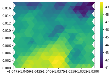
Here, we select a 1° x 1° region such that we’ll have a chance to actually see some triangles. In ICON terminology, a triangle is a “cell”. So we can select our desired triangles based on the cell-latitude and cell-logitude.
mask = (
    (ds.clat.values > np.deg2rad(0))
    & (ds.clat.values < np.deg2rad(1))
    & (ds.clon.values > np.deg2rad(-60))
    & (ds.clon.values < np.deg2rad(-59))
)
For each of the selected cell, we need the indices of the three corners of the triangles (the tris array from above). In ICON grid files, this array is called vertex_of_cell. It also is transposed and uses Fortran-indexing (which starts counting by one). Let’s load this array for our selected region and correct for the index offset:
voc = ds.vertex_of_cell.T[mask].values - 1
We also want to know the bounding box of our triangles to properly set the extent of our plot. We could use the range which we used above to select our triangles, but then we couldn’t apply the example to other selections. Furthermore, here we are interested in the bounding box of the triangle corners not the triangle centers.
So what we’ll do is to find out which vertices actually are used by any of the selected triangles:
used_vertices = np.unique(voc)
Now we can compute the extent of our plot:
lat_min = ds.vlat[used_vertices].min().values
lat_max = ds.vlat[used_vertices].max().values
lon_min = ds.vlon[used_vertices].min().values
lon_max = ds.vlon[used_vertices].max().values
Now, we are all set and can do our little plot.
plt.tripcolor(ds.vlon, ds.vlat, voc, ds.prw.isel(time=100, cell=mask).values)
plt.xlim(lon_min, lon_max)
plt.ylim(lat_min, lat_max)
plt.colorbar()
<matplotlib.colorbar.Colorbar at 0x2b80afa4b8e0>