Resampling to lon-lat grid

This notebook shows a quick way to resample HEALPix data to a lon/lat grid using nearest neighbors.

Remapping via source indices

Likely, the easiest method for resampling HEALPix data is to compute which index of the HEALPix grid corresponds to each pixel of the target grid. We’ll take this approach and build a function which computes the HEALPix pixel indices for each lon/lat pair in a rectilinear grid of longitudes and latitudes:

import numpy as np
import xarray as xr
import healpy


def get_nn_lon_lat_index(nside, lons, lats):
    lons2, lats2 = np.meshgrid(lons, lats)
    return xr.DataArray(
        healpy.ang2pix(nside, lons2, lats2, nest=True, lonlat=True),
        coords=[("lat", lats), ("lon", lons)],
    )

Let’s try this function on a coarse HEALPix grid (nside=2) and for a coarse global lon/lat grid. We’ll obtain an array of cell indices:

get_nn_lon_lat_index(2, np.linspace(-180, 180, 10), np.linspace(-90, 90, 5))

<xarray.DataArray (lat: 5, lon: 10)>
array([[40, 40, 40, 44, 44, 32, 32, 36, 36, 40],
       [42, 42, 41, 46, 45, 34, 33, 38, 37, 42],
       [25, 25, 30, 29, 18, 17, 22, 21, 26, 25],
       [10, 10,  9, 14, 13,  2,  1,  6,  5, 10],
       [11, 11, 11, 15, 15,  3,  3,  7,  7, 11]])
Coordinates:
  * lat      (lat) float64 -90.0 -45.0 0.0 45.0 90.0
  * lon      (lon) float64 -180.0 -140.0 -100.0 -60.0 ... 60.0 100.0 140.0 180.0

xarray.DataArray

• lat: 5
• lon: 10

• 40 40 40 44 44 32 32 36 36 40 42 42 ... 5 10 11 11 11 15 15 3 3 7 7 11

  array([[40, 40, 40, 44, 44, 32, 32, 36, 36, 40],
         [42, 42, 41, 46, 45, 34, 33, 38, 37, 42],
         [25, 25, 30, 29, 18, 17, 22, 21, 26, 25],
         [10, 10,  9, 14, 13,  2,  1,  6,  5, 10],
         [11, 11, 11, 15, 15,  3,  3,  7,  7, 11]])

• Coordinates: (2)
  • lat
    (lat)
    float64
    -90.0 -45.0 0.0 45.0 90.0

    array([-90., -45.,   0.,  45.,  90.])

  • lon
    (lon)
    float64
    -180.0 -140.0 ... 140.0 180.0

    array([-180., -140., -100.,  -60.,  -20.,   20.,   60.,  100.,  140.,  180.])

• Indexes: (2)
  • lat
    PandasIndex

    PandasIndex(Index([-90.0, -45.0, 0.0, 45.0, 90.0], dtype='float64', name='lat'))

  • lon
    PandasIndex

    PandasIndex(Index([-180.0, -140.0, -100.0, -60.0, -20.0, 20.0, 60.0, 100.0, 140.0, 180.0], dtype='float64', name='lon'))

• Attributes: (0)

This doesn’t look too bad (we expect values in the range of \(0\) to \(12 N_\rm{side}^2-1\) or \(0\) to \(47\) in this case). But let’s also check this result visually with a few more pixels:

get_nn_lon_lat_index(2, np.linspace(-180, 180, 800), np.linspace(-90, 90, 400)).plot(
    figsize=(8, 4)
)
None

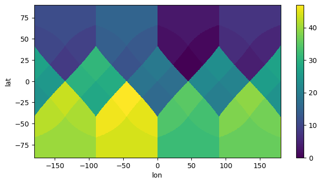
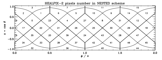
Indeed, this shows us the HEALPix pixel numbers on a lon/lat grid as depicted in Górski et al., 2004:

This seems to be correct, so let’s apply it to some model output:

Remapping model output

Of course, we first need access to some model output:

import intake

cat = intake.open_catalog("https://data.nextgems-h2020.eu/catalog.yaml")

When selecting the zoom level, it’s best to find a level which approximately matches your desired output resolution. Please have a look at the HEALPix intro for a comparison between angular resolution and typical HEALPix zoom levels. In this case, we have an angular resolution of about 0.05°, so zoom=10 is probably appropriate.

zoom = 10
ds = cat.ICON.ngc3028(zoom=zoom, time="PT30M").to_dask()

Now that we have the output available, let’s compute remapping indices for a region including the Amazon and the Caribbean:

idx = get_nn_lon_lat_index(
    2**zoom, np.linspace(-70, -55, 300), np.linspace(5, 20, 300)
)

We can now use the index to select from the cell dimension to obtain a new xr.DataArray with surface temperature on a lon lat grid:

tas_lon_lat = ds.tas.isel(time=0, cell=idx)
tas_lon_lat

<xarray.DataArray 'tas' (lat: 300, lon: 300)>
[90000 values with dtype=float32]
Coordinates:
    time     datetime64[ns] 2020-01-20T00:30:00
  * lat      (lat) float64 5.0 5.05 5.1 5.151 5.201 ... 19.85 19.9 19.95 20.0
  * lon      (lon) float64 -70.0 -69.95 -69.9 -69.85 ... -55.1 -55.05 -55.0
Attributes:
    cell_methods:   time: point
    component:      atmo
    grid_mapping:   crs
    long_name:      temperature in 2m
    standard_name:  air_temperature
    units:          K
    vgrid:          height_2m

xarray.DataArray

'tas'

• lat: 300
• lon: 300

• ...

  [90000 values with dtype=float32]

• Coordinates: (3)
  • time
    ()
    datetime64[ns]
    2020-01-20T00:30:00

    axis :

    T

    array('2020-01-20T00:30:00.000000000', dtype='datetime64[ns]')

  • lat
    (lat)
    float64
    5.0 5.05 5.1 ... 19.9 19.95 20.0

    array([ 5.      ,  5.050167,  5.100334, ..., 19.899666, 19.949833, 20.      ])

  • lon
    (lon)
    float64
    -70.0 -69.95 -69.9 ... -55.05 -55.0

    array([-70.      , -69.949833, -69.899666, ..., -55.100334, -55.050167,
           -55.      ])

• Indexes: (2)
  • lat
    PandasIndex

    PandasIndex(Index([               5.0,  5.050167224080267, 5.1003344481605355,
            5.150501672240803,   5.20066889632107,  5.250836120401337,
            5.301003344481606,  5.351170568561873,   5.40133779264214,
            5.451505016722408,
           ...
           19.548494983277592,  19.59866220735786, 19.648829431438127,
           19.698996655518393,  19.74916387959866,  19.79933110367893,
             19.8494983277592, 19.899665551839465,  19.94983277591973,
                         20.0],
          dtype='float64', name='lat', length=300))

  • lon
    PandasIndex

    PandasIndex(Index([             -70.0, -69.94983277591973, -69.89966555183946,
           -69.84949832775919, -69.79933110367892, -69.74916387959867,
            -69.6989966555184, -69.64882943143813, -69.59866220735786,
           -69.54849498327759,
           ...
           -55.45150501672241, -55.40133779264214, -55.35117056856187,
           -55.30100334448161, -55.25083612040134, -55.20066889632107,
            -55.1505016722408, -55.10033444816054, -55.05016722408027,
                        -55.0],
          dtype='float64', name='lon', length=300))

• Attributes: (7)

  cell_methods :

  time: point

  component :

  atmo

  grid_mapping :

  crs

  long_name :

  temperature in 2m

  standard_name :

  air_temperature

  units :

  K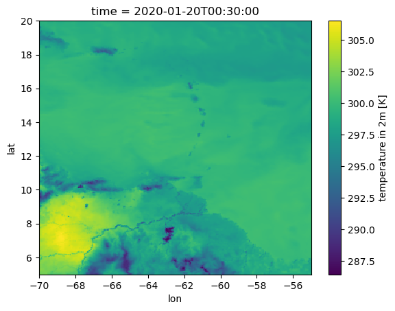

  vgrid :

  height_2m

As the data is now on a rectangular grid, we can plot it quite easily:

tas_lon_lat.plot()
None

Anti-Aliasing

Nearest-Neighbor remapping can lead to aliasing: along steep gradients (e.g. the temperature difference between land and water along the Amazon river), data is picked seemingly randomly from either side of the gradient (it depends on how the source and target grids fit onto each other on the very fine scale). While this effect likely averages out when analyzing larger areas, it can disturb the local scale. Several methods exist to overcome this problem. A simple approximative way is supersampling, where we first interpolate to a finer grid and then average the interpolated data back to our target grid. Uniform supersampling can be implemented as follows:

supersampling = {"lon": 4, "lat": 4}
idx = get_nn_lon_lat_index(
    2**zoom,
    np.linspace(-70, -55, supersampling["lon"] * 300),
    np.linspace(5, 20, supersampling["lat"] * 300),
)
tas_lon_lat_aa = ds.tas.isel(time=0, cell=idx).coarsen(supersampling).mean()
tas_lon_lat_aa.plot()
None

While the output barely changes for uniform areas, regions with gradients apprear much smoother now.

Saving to disk

Of course, any data remapped this way can be saved to disk by the usual means of xarray I/O methods, including netCDF and zarr formats. If data is opened using dask (remember to use some chunks definition while opening), it is possible to perform the regridding lazily, chunk by chunk while writing the output.

Selecting zoom level automatically

If we want a simple automatic way of selecting an appropriate zoom level, we can also compute HEALPix indices for multiple zoom levels and observe how many unique index values we obtain:

• If we have only a few unique values, a single model output pixel will end up in many pixels in the lon/lat projection: the HEALPix resolution is too coarse for the desired lon/lat grid.

• If we have as many unique values as lon/lat pixels, every lon/lat pixel will get data from a different model output pixel, but we might skip a bunch of model pixels, thus subsample the output and might see aliasing effects.

So to choose an appropriate zoom level, we might want to search for the zoom where the unique_fraction goes towards 1 but not necessarily be exactly 1.

Selecting a good zoom level comes with multiple advantages:

• We don’t load excessive amounts of data -> our code becomes faster

• Using pre-aggregated data can reduce aliasing effects (if the output hierarchy uses area averaging)

@lambda f: np.vectorize(f, excluded={1, 2})
def unique_fraction(nside, lons, lats):
    idx = get_nn_lon_lat_index(nside, lons, lats)
    return np.unique(idx).size / idx.size

Let’s try this function for several zoom levels and different grids:

import matplotlib.pylab as plt

zoom = np.arange(15)

grids = [
    (np.linspace(-70, -55, 300), np.linspace(5, 20, 300), "Carribean, fine"),
    (np.linspace(-70, -55, 100), np.linspace(5, 20, 100), "Carribean, coarse"),
    (np.linspace(-180, 180, 360), np.linspace(-90, 90, 180), "Globe, 1° by 1°"),
]

for lons, lats, label in grids:
    plt.plot(zoom, unique_fraction(2**zoom, lons, lats), label=label)

plt.xlabel("zoom")
plt.ylabel("unique fraction")
plt.legend()
None

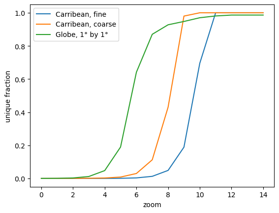
As the change between 0 and 1 typically is rather steep, we could get a simple criterion for “approaching 1” by just picking the first zoom level where unique_fraction > 0.5 and use that as a suggested zoom level:

for lons, lats, label in grids:
    print(f"{label:30s} {np.argmax(unique_fraction(2**zoom, lons, lats) > 0.5)}")

Carribean, fine                10
Carribean, coarse              9
Globe, 1° by 1°                6

So based on this criterion, the best zoom level for our initial example would indeed be 10. We can also see that level 6 could be appropriate for a global 1° by 1° grid as suggested in the HEALPix intro.