Grid Index Ordering

Cell indices in ICON global grids are ordered in a specific manner which simplifies a bunch of operations an which is interesting to know about. Here, we’ll look at a few aspects of this particular ordering.

%matplotlib inline
import matplotlib.pylab as plt
import numpy as np
import xarray as xr
import cartopy.crs as ccrs
import cartopy.feature as cfeature

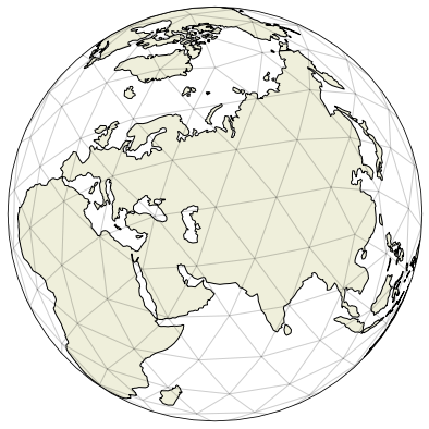
We’ll start using a relatively coarse (R02B03) grid in order to make the plots less crowded and our live easier.

grid = xr.open_dataset(
    "/pool/data/ICON/grids/public/mpim/0030/icon_grid_0030_R02B03_G.nc"
)
grid

<xarray.Dataset>
Dimensions:                         (cell: 5120, nv: 3, vertex: 2562, ne: 6, edge: 7680, no: 4, nc: 2, max_stored_decompositions: 4, two_grf: 2, cell_grf: 14, max_chdom: 1, edge_grf: 24, vert_grf: 13)
Coordinates:
    clon                            (cell) float64 1.274 1.34 ... 1.437 1.329
    clat                            (cell) float64 0.9184 0.9398 ... -0.8052
    vlon                            (vertex) float64 1.274 1.213 ... 1.274 1.325
    vlat                            (vertex) float64 0.9625 0.8955 ... -0.7609
    elon                            (edge) float64 1.306 1.242 ... 1.407 1.354
    elat                            (edge) float64 0.9292 0.9292 ... -0.7939
Dimensions without coordinates: cell, nv, vertex, ne, edge, no, nc, max_stored_decompositions, two_grf, cell_grf, max_chdom, edge_grf, vert_grf
Data variables: (12/91)
    clon_vertices                   (cell, nv) float64 1.274 1.213 ... 1.325
    clat_vertices                   (cell, nv) float64 0.9625 0.8955 ... -0.7609
    vlon_vertices                   (vertex, ne) float64 9.969e+36 ... 9.969e+36
    vlat_vertices                   (vertex, ne) float64 9.969e+36 ... 9.969e+36
    elon_vertices                   (edge, no) float64 1.335 1.34 ... 1.385
    elat_vertices                   (edge, no) float64 0.8955 0.9398 ... -0.8265
    ...                              ...
    edge_dual_normal_cartesian_x    (edge) float64 -0.2769 -0.6793 ... 0.6559
    edge_dual_normal_cartesian_y    (edge) float64 0.8043 -0.512 ... 0.4705
    edge_dual_normal_cartesian_z    (edge) float64 -0.5257 0.5257 ... 0.5902
    cell_circumcenter_cartesian_x   (cell) float64 0.1775 0.1351 ... 0.1662
    cell_circumcenter_cartesian_y   (cell) float64 0.5805 0.5743 ... 0.6727
    cell_circumcenter_cartesian_z   (cell) float64 0.7947 0.8074 ... -0.721
Attributes: (12/43)
    title:                    ICON grid description
    institution:              Max Planck Institute for Meteorology/Deutscher ...
    source:                   git@git.mpimet.mpg.de:GridGenerator.git
    revision:                 2cdf99bec403902989148ebb4bd38c218a64a1b3
    date:                     20190405 at 141502
    user_name:                Rene Redler (m300083)
    ...                       ...
    topography:               modified SRTM30
    symmetry:                 along equator
    subcentre:                1
    number_of_grid_used:      30
    ICON_grid_file_uri:       http://icon-downloads.mpimet.mpg.de/grids/publi...
    NCO:                      netCDF Operators version 4.7.5 (Homepage = http...

We’ll use this little function which displays our selected grid cells on a map. It uses

• voc (vertex of cell), which lists the vertices of each cell, in Fortran (1-based) index convention

• clat and clon: coordinates of cell centers

• vlat and vlon: coordinates of vertices

The function draws a line along the cell centers in index order and colors the centers also in this order.

def show_grid(voc, clat, clon, vlat, vlon):
    fig = plt.figure(figsize=(14, 7))
    ax = fig.add_subplot(1, 1, 1, projection=ccrs.Orthographic(60, 45))
    ax.set_global()
    ax.add_feature(cfeature.LAND, zorder=0, edgecolor="black")

    plt.plot(np.rad2deg(clon), np.rad2deg(clat), transform=ccrs.Geodetic())
    plt.scatter(
        np.rad2deg(clon),
        np.rad2deg(clat),
        c=np.arange(len(clon)),
        s=15,
        zorder=10,
        cmap="turbo",
        transform=ccrs.Geodetic(),
    )
    for v1, v2, v3 in voc.T - 1:
        i = np.array([v1, v2, v3, v1])
        plt.plot(
            np.rad2deg(vlon[i]),
            np.rad2deg(vlat[i]),
            c="k",
            lw=1,
            alpha=0.1,
            transform=ccrs.Geodetic(),
        )
    plt.colorbar(label="cell index")
    plt.show()
    plt.close()

As we can not see anything on the backside of the globe anyways and an we know that the ICON grid is based on an icosahedron, we’ll cut out one of the faces of the icosahedron to look at the internal grid structure. We’ll call this subgrid sg1.

sg1 = grid.isel(cell=slice(2 ** (2 * 4)))
show_grid(
    sg1.vertex_of_cell.values,
    sg1.clat.values,
    sg1.clon.values,
    grid.vlat.values,
    grid.vlon.values,
)

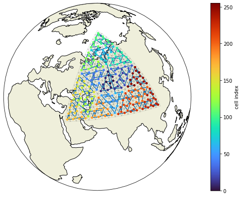
We observe that the central triangle of any larger (composed) triangle is always the first index within that group. Or the other way around: four triangles form one larger triangle and every four triangles are ordered as [center, corner1, corner2, corner3].

Let’s have a look into the vertex indices of four such connected triangles (we’ll use the first, most central triangles for the example):

sg1.vertex_of_cell.values.T[0:4]

array([[1, 2, 3],
       [3, 4, 1],
       [1, 5, 2],
       [2, 6, 3]], dtype=int32)

Each row in this array represents one triangle and each column shows the indices of the vertices within that triangle.

We know that lower three triangles are the three corner triangles and we can see that in each triangle, the middle vertex occurs only once. As only the outer vertices of the larger triangle composed by these small triangles are not shared between inner triangles, these vertices must be the outer vertices of the larger (connected) triangle. Let’s use this information to coarsen our grid.

def coarsen_vertex_of_cell(voc):
    return voc.reshape(3, -1, 4)[1, :, 1:].T

The function above reshapes the voc array into a stack of these 3x4 blocks of vertex indices and then just cuts out our three corner indices into a new, coarser voc-array.

Let’s also define a function which we can use to coarsen cell center values (e.g. clat and clon) by selecting the value of the central (first) triangle:

def coarsen_cell_center(cvalue):
    return cvalue[..., ::4]

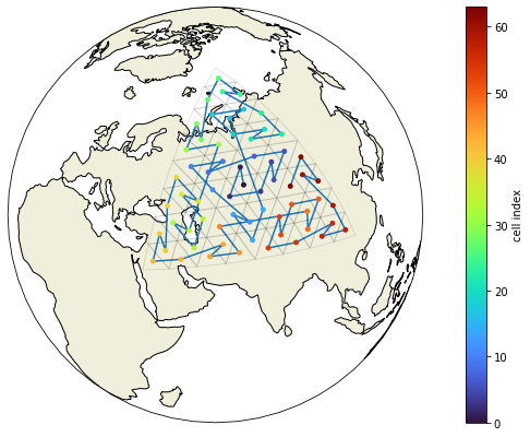
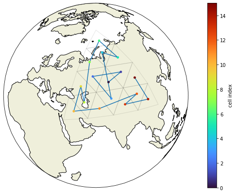
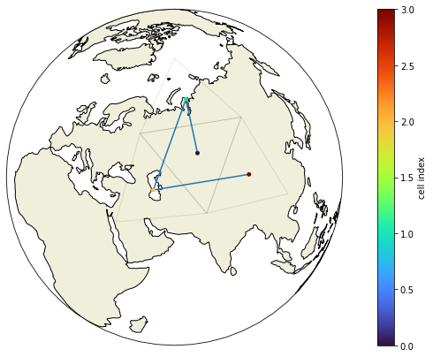
We can now apply these functions recursively to coarsen the grid several times and have a look at the resulting grid structures:

voc = sg1.vertex_of_cell.values
clat = sg1.clat.values
clon = sg1.clon.values
for i in range(3):
    voc = coarsen_vertex_of_cell(voc)
    clat = coarsen_cell_center(clat)
    clon = coarsen_cell_center(clon)
    show_grid(voc, clat, clon, grid.vlat.values, grid.vlon.values)

Here’s a little test which would print out the coarsening level and the cell index of any group of triangles which would violate out assumption about the ordering of the vertices. As it doesn’t print anything, we know that the method works for this grid.

voc = sg1.vertex_of_cell.values
for l in range(4):
    for i, g in enumerate(voc.reshape(3, -1, 4).transpose(1, 0, 2)):
        if np.any(g[:, 0, np.newaxis] == g[1, 1:]):
            print(l, i, g)
    voc = coarsen_vertex_of_cell(voc)

We can also apply the coarsening several times to our full grid to make a little image of the grid structure on the globe:

voc = coarsen_vertex_of_cell(coarsen_vertex_of_cell(grid.vertex_of_cell.values))

fig = plt.figure(figsize=(14, 7))
ax = fig.add_subplot(1, 1, 1, projection=ccrs.Orthographic(60, 45))
ax.set_global()
ax.add_feature(cfeature.LAND, zorder=0, edgecolor="black")

for v1, v2, v3 in voc.T - 1:
    i = np.array([v1, v2, v3, v1])
    plt.plot(
        np.rad2deg(grid.vlon.values[i]),
        np.rad2deg(grid.vlat.values[i]),
        c="k",
        lw=1,
        alpha=0.1,
        transform=ccrs.Geodetic(),
    )
plt.show()
plt.close()