
Selecting and Reindexing of Area of Interest#
The elegant way of dealing with large output#
Before working through this script, it is helpful to have had a look into Triangular Meshes and Basic Plotting to get a basic understanding of plotting on a triangular basis.
Three-dimensional global ICON output for example requires many times more memory than two-dimensional output. The handling of such large amounts of data can very quickly lead to the exhaustion of the given memory. If you are sitting right next to a supercomputer, you are tempted to just request more RAM and go for it. However, there are elegant solutions besides the powerful one and since a lot of RAM also means a lot of electricity and a lot of coolant, the motivation for an elegant way is also to save limited resources.
In many cases, we rarely look at the complete global output, but rather at a specific, selected area. It is therefore advisable to cut out only this area. For this purpose it is very helpful to reduce the grid information from the global grid file to the area of interest but in such a way that the indexing makes sense starting at 0 and counting up continuously. The advantage is that we generate a new local grid-file, which looks like the global grid-file but is much smaller in terms of storage capacity and therefore easier and faster to handle.
So let’s do something for the climate 🌍 and first of all load the necessary libraries and the global grid-file:
import xarray as xr
import numpy as np
Importing the Grid-File#
grid = xr.open_dataset(
    "/work/mh0287/k203123/Dyamond++/icon-aes-dyw2/experiments/dpp0029/icon_grid_0015_R02B09_G.nc"
)
grid
<xarray.Dataset>
Dimensions:                         (cell: 20971520, nv: 3, vertex: 10485762,
                                     ne: 6, edge: 31457280, no: 4, nc: 2,
                                     max_stored_decompositions: 4, two_grf: 2,
                                     cell_grf: 14, max_chdom: 1, edge_grf: 24,
                                     vert_grf: 13)
Coordinates:
    clon                            (cell) float64 ...
    clat                            (cell) float64 ...
    vlon                            (vertex) float64 ...
    vlat                            (vertex) float64 ...
    elon                            (edge) float64 ...
    elat                            (edge) float64 ...
Dimensions without coordinates: cell, nv, vertex, ne, edge, no, nc,
                                max_stored_decompositions, two_grf, cell_grf,
                                max_chdom, edge_grf, vert_grf
Data variables: (12/91)
    clon_vertices                   (cell, nv) float64 ...
    clat_vertices                   (cell, nv) float64 ...
    vlon_vertices                   (vertex, ne) float64 ...
    vlat_vertices                   (vertex, ne) float64 ...
    elon_vertices                   (edge, no) float64 ...
    elat_vertices                   (edge, no) float64 ...
    ...                              ...
    edge_dual_normal_cartesian_x    (edge) float64 ...
    edge_dual_normal_cartesian_y    (edge) float64 ...
    edge_dual_normal_cartesian_z    (edge) float64 ...
    cell_circumcenter_cartesian_x   (cell) float64 ...
    cell_circumcenter_cartesian_y   (cell) float64 ...
    cell_circumcenter_cartesian_z   (cell) float64 ...
Attributes: (12/43)
    title:                    ICON grid description
    institution:              Max Planck Institute for Meteorology/Deutscher ...
    source:                   git@git.mpimet.mpg.de:GridGenerator.git
    revision:                 d00fcac1f61fa16c686bfe51d1d8eddd09296cb5
    date:                     20180529 at 222250
    user_name:                Rene Redler (m300083)
    ...                       ...
    topography:               modified SRTM30
    subcentre:                1
    number_of_grid_used:      15
    history:                  Thu Aug 16 11:05:44 2018: ncatted -O -a ICON_gr...
    ICON_grid_file_uri:       http://icon-downloads.mpimet.mpg.de/grids/publi...
NCO: netCDF Operators version 4.7.5 (Homepage = http...- cell: 20971520
- nv: 3
- vertex: 10485762
- ne: 6
- edge: 31457280
- no: 4
- nc: 2
- max_stored_decompositions: 4
- two_grf: 2
- cell_grf: 14
- max_chdom: 1
- edge_grf: 24
- vert_grf: 13
- clon(cell)float64...
- long_name :
- center longitude
- units :
- radian
- standard_name :
- grid_longitude
- bounds :
- clon_vertices
[20971520 values with dtype=float64]
- clat(cell)float64...
- long_name :
- center latitude
- units :
- radian
- standard_name :
- grid_latitude
- bounds :
- clat_vertices
[20971520 values with dtype=float64]
- vlon(vertex)float64...
- long_name :
- vertex longitude
- units :
- radian
- standard_name :
- grid_longitude
- bounds :
- vlon_vertices
[10485762 values with dtype=float64]
- vlat(vertex)float64...
- long_name :
- vertex latitude
- units :
- radian
- standard_name :
- grid_latitude
- bounds :
- vlat_vertices
[10485762 values with dtype=float64]
- elon(edge)float64...
- long_name :
- edge midpoint longitude
- units :
- radian
- standard_name :
- grid_longitude
- bounds :
- elon_vertices
[31457280 values with dtype=float64]
- elat(edge)float64...
- long_name :
- edge midpoint latitude
- units :
- radian
- standard_name :
- grid_latitude
- bounds :
- elat_vertices
[31457280 values with dtype=float64]
- clon_vertices(cell, nv)float64...
- units :
- radian
[62914560 values with dtype=float64]
- clat_vertices(cell, nv)float64...
- units :
- radian
[62914560 values with dtype=float64]
- vlon_vertices(vertex, ne)float64...
- units :
- radian
[62914572 values with dtype=float64]
- vlat_vertices(vertex, ne)float64...
- units :
- radian
[62914572 values with dtype=float64]
- elon_vertices(edge, no)float64...
- units :
- radian
[125829120 values with dtype=float64]
- elat_vertices(edge, no)float64...
- units :
- radian
[125829120 values with dtype=float64]
- ifs2icon_cell_grid(cell)float64...
- long_name :
- ifs to icon cells
[20971520 values with dtype=float64]
- ifs2icon_edge_grid(edge)float64...
- long_name :
- ifs to icon edge
[31457280 values with dtype=float64]
- ifs2icon_vertex_grid(vertex)float64...
- long_name :
- ifs to icon vertex
[10485762 values with dtype=float64]
- cell_area(cell)float64...
- long_name :
- area of grid cell
- units :
- m2
- standard_name :
- area
- grid_type :
- unstructured
- number_of_grid_in_reference :
- 1
[20971520 values with dtype=float64]
- dual_area(vertex)float64...
- long_name :
- areas of dual hexagonal/pentagonal cells
- units :
- m2
- standard_name :
- area
[10485762 values with dtype=float64]
- phys_cell_id(cell)int32...
- long_name :
- physical domain ID of cell
- grid_type :
- unstructured
- number_of_grid_in_reference :
- 1
[20971520 values with dtype=int32]
- phys_edge_id(edge)int32...
- long_name :
- physical domain ID of edge
[31457280 values with dtype=int32]
- lon_cell_centre(cell)float64...
- long_name :
- longitude of cell centre
- units :
- radian
- grid_type :
- unstructured
- number_of_grid_in_reference :
- 1
[20971520 values with dtype=float64]
- lat_cell_centre(cell)float64...
- long_name :
- latitude of cell centre
- units :
- radian
- grid_type :
- unstructured
- number_of_grid_in_reference :
- 1
[20971520 values with dtype=float64]
- lat_cell_barycenter(cell)float64...
- long_name :
- latitude of cell barycenter
- units :
- radian
- grid_type :
- unstructured
- number_of_grid_in_reference :
- 1
[20971520 values with dtype=float64]
- lon_cell_barycenter(cell)float64...
- long_name :
- longitude of cell barycenter
- units :
- radian
- grid_type :
- unstructured
- number_of_grid_in_reference :
- 1
[20971520 values with dtype=float64]
- longitude_vertices(vertex)float64...
- long_name :
- longitude of vertices
- units :
- radian
[10485762 values with dtype=float64]
- latitude_vertices(vertex)float64...
- long_name :
- latitude of vertices
- units :
- radian
[10485762 values with dtype=float64]
- lon_edge_centre(edge)float64...
- long_name :
- longitudes of edge midpoints
- units :
- radian
[31457280 values with dtype=float64]
- lat_edge_centre(edge)float64...
- long_name :
- latitudes of edge midpoints
- units :
- radian
[31457280 values with dtype=float64]
- edge_of_cell(nv, cell)int32...
- long_name :
- edges of each cellvertices
[62914560 values with dtype=int32]
- vertex_of_cell(nv, cell)int32...
- long_name :
- vertices of each cellcells ad
[62914560 values with dtype=int32]
- adjacent_cell_of_edge(nc, edge)int32...
- long_name :
- cells adjacent to each edge
[62914560 values with dtype=int32]
- edge_vertices(nc, edge)int32...
- long_name :
- vertices at the end of of each edge
[62914560 values with dtype=int32]
- cells_of_vertex(ne, vertex)int32...
- long_name :
- cells around each vertex
[62914572 values with dtype=int32]
- edges_of_vertex(ne, vertex)int32...
- long_name :
- edges around each vertex
[62914572 values with dtype=int32]
- vertices_of_vertex(ne, vertex)int32...
- long_name :
- vertices around each vertex
[62914572 values with dtype=int32]
- cell_area_p(cell)float64...
- long_name :
- area of grid cell
- units :
- m2
- grid_type :
- unstructured
- number_of_grid_in_reference :
- 1
[20971520 values with dtype=float64]
- cell_elevation(cell)float64...
- long_name :
- elevation at the cell centers
- units :
- m
- grid_type :
- unstructured
- number_of_grid_in_reference :
- 1
[20971520 values with dtype=float64]
- cell_sea_land_mask(cell)int32...
- long_name :
- sea (-2 inner, -1 boundary) land (2 inner, 1 boundary) mask for the cell
- units :
- 2,1,-1,-
- grid_type :
- unstructured
- number_of_grid_in_reference :
- 1
[20971520 values with dtype=int32]
- cell_domain_id(cell, max_stored_decompositions)int32...
- long_name :
- cell domain id for decomposition
[83886080 values with dtype=int32]
- cell_no_of_domains(max_stored_decompositions)int32...
- long_name :
- number of domains for each decomposition
array([0, 0, 0, 0], dtype=int32)
- dual_area_p(vertex)float64...
- long_name :
- areas of dual hexagonal/pentagonal cells
- units :
- m2
[10485762 values with dtype=float64]
- edge_length(edge)float64...
- long_name :
- lengths of edges of triangular cells
- units :
- m
[31457280 values with dtype=float64]
- edge_cell_distance(nc, edge)float64...
- long_name :
- distances between edge midpoint and adjacent triangle midpoints
- units :
- m
[62914560 values with dtype=float64]
- dual_edge_length(edge)float64...
- long_name :
- lengths of dual edges (distances between triangular cell circumcenters)
- units :
- m
[31457280 values with dtype=float64]
- edgequad_area(edge)float64...
- long_name :
- area around the edge formed by the two adjacent triangles
- units :
- m2
[31457280 values with dtype=float64]
- edge_elevation(edge)float64...
- long_name :
- elevation at the edge centers
- units :
- m
[31457280 values with dtype=float64]
- edge_sea_land_mask(edge)int32...
- long_name :
- sea (-2 inner, -1 boundary) land (2 inner, 1 boundary) mask for the cell
- units :
- 2,1,-1,-
[31457280 values with dtype=int32]
- edge_vert_distance(nc, edge)float64...
- long_name :
- distances between edge midpoint and vertices of that edge
- units :
- m
[62914560 values with dtype=float64]
- zonal_normal_primal_edge(edge)float64...
- long_name :
- zonal component of normal to primal edge
- units :
- radian
[31457280 values with dtype=float64]
- meridional_normal_primal_edge(edge)float64...
- long_name :
- meridional component of normal to primal edge
- units :
- radian
[31457280 values with dtype=float64]
- zonal_normal_dual_edge(edge)float64...
- long_name :
- zonal component of normal to dual edge
- units :
- radian
[31457280 values with dtype=float64]
- meridional_normal_dual_edge(edge)float64...
- long_name :
- meridional component of normal to dual edge
- units :
- radian
[31457280 values with dtype=float64]
- orientation_of_normal(nv, cell)int32...
- long_name :
- orientations of normals to triangular cell edges
[62914560 values with dtype=int32]
- cell_index(cell)int32...
- long_name :
- cell index
[20971520 values with dtype=int32]
- parent_cell_index(cell)int32...
- long_name :
- parent cell index
[20971520 values with dtype=int32]
- parent_cell_type(cell)int32...
- long_name :
- parent cell type
[20971520 values with dtype=int32]
- neighbor_cell_index(nv, cell)int32...
- long_name :
- cell neighbor index
[62914560 values with dtype=int32]
- child_cell_index(no, cell)int32...
- long_name :
- child cell index
[83886080 values with dtype=int32]
- child_cell_id(cell)int32...
- long_name :
- domain ID of child cell
[20971520 values with dtype=int32]
- edge_index(edge)int32...
- long_name :
- edge index
[31457280 values with dtype=int32]
- edge_parent_type(edge)int32...
- long_name :
- edge paren
[31457280 values with dtype=int32]
- vertex_index(vertex)int32...
- long_name :
- vertices index
[10485762 values with dtype=int32]
- edge_orientation(ne, vertex)int32...
- long_name :
- edge orientation
[62914572 values with dtype=int32]
- edge_system_orientation(edge)int32...
- long_name :
- edge system orientation
[31457280 values with dtype=int32]
- refin_c_ctrl(cell)int32...
- long_name :
- refinement control flag for cells
[20971520 values with dtype=int32]
- index_c_list(two_grf, cell_grf)int32...
- long_name :
- list of start and end indices for each refinement control level for cells
array([[-2147483647, -2147483647, -2147483647, -2147483647, -2147483647, -2147483647, -2147483647, -2147483647, -2147483647, -2147483647, -2147483647, -2147483647, -2147483647, -2147483647], [-2147483647, -2147483647, -2147483647, -2147483647, -2147483647, -2147483647, -2147483647, -2147483647, -2147483647, -2147483647, -2147483647, -2147483647, -2147483647, -2147483647]], dtype=int32) - start_idx_c(max_chdom, cell_grf)int32...
- long_name :
- list of start indices for each refinement control level for cells
array([[20971521, 20971521, 20971521, 20971521, 20971521, 20971521, 20971521, 20971521, 20971521, 1, 1, 1, 1, 1]], dtype=int32) - end_idx_c(max_chdom, cell_grf)int32...
- long_name :
- list of end indices for each refinement control level for cells
array([[20971520, 20971520, 20971520, 20971520, 20971520, 20971520, 20971520, 20971520, 20971520, 0, 0, 0, 0, 0]], dtype=int32) - refin_e_ctrl(edge)int32...
- long_name :
- refinement control flag for edges
[31457280 values with dtype=int32]
- index_e_list(two_grf, edge_grf)int32...
- long_name :
- list of start and end indices for each refinement control level for edges
array([[-2147483647, -2147483647, -2147483647, -2147483647, -2147483647, -2147483647, -2147483647, -2147483647, -2147483647, -2147483647, -2147483647, -2147483647, -2147483647, -2147483647, -2147483647, -2147483647, -2147483647, -2147483647, -2147483647, -2147483647, -2147483647, -2147483647, -2147483647, -2147483647], [-2147483647, -2147483647, -2147483647, -2147483647, -2147483647, -2147483647, -2147483647, -2147483647, -2147483647, -2147483647, -2147483647, -2147483647, -2147483647, -2147483647, -2147483647, -2147483647, -2147483647, -2147483647, -2147483647, -2147483647, -2147483647, -2147483647, -2147483647, -2147483647]], dtype=int32) - start_idx_e(max_chdom, edge_grf)int32...
- long_name :
- list of start indices for each refinement control level for edges
array([[31457281, 31457281, 31457281, 31457281, 31457281, 31457281, 31457281, 31457281, 31457281, 31457281, 31457281, 31457281, 31457281, 31457281, 1, 1, 1, 1, 1, 1, 1, 1, 1, 1]], dtype=int32) - end_idx_e(max_chdom, edge_grf)int32...
- long_name :
- list of end indices for each refinement control level for edges
array([[31457280, 31457280, 31457280, 31457280, 31457280, 31457280, 31457280, 31457280, 31457280, 31457280, 31457280, 31457280, 31457280, 31457280, 0, 0, 0, 0, 0, 0, 0, 0, 0, 0]], dtype=int32) - refin_v_ctrl(vertex)int32...
- long_name :
- refinement control flag for vertices
[10485762 values with dtype=int32]
- index_v_list(two_grf, vert_grf)int32...
- long_name :
- list of start and end indices for each refinement control level for vertices
array([[-2147483647, -2147483647, -2147483647, -2147483647, -2147483647, -2147483647, -2147483647, -2147483647, -2147483647, -2147483647, -2147483647, -2147483647, -2147483647], [-2147483647, -2147483647, -2147483647, -2147483647, -2147483647, -2147483647, -2147483647, -2147483647, -2147483647, -2147483647, -2147483647, -2147483647, -2147483647]], dtype=int32) - start_idx_v(max_chdom, vert_grf)int32...
- long_name :
- list of start indices for each refinement control level for vertices
array([[10485763, 10485763, 10485763, 10485763, 10485763, 10485763, 10485763, 10485763, 1, 1, 1, 1, 1]], dtype=int32) - end_idx_v(max_chdom, vert_grf)int32...
- long_name :
- list of end indices for each refinement control level for vertices
array([[10485762, 10485762, 10485762, 10485762, 10485762, 10485762, 10485762, 10485762, 0, 0, 0, 0, 0]], dtype=int32) - parent_edge_index(edge)int32...
- long_name :
- parent edge index
[31457280 values with dtype=int32]
- child_edge_index(no, edge)int32...
- long_name :
- child edge index
[125829120 values with dtype=int32]
- child_edge_id(edge)int32...
- long_name :
- domain ID of child edge
[31457280 values with dtype=int32]
- parent_vertex_index(vertex)int32...
- long_name :
- parent vertex index
[10485762 values with dtype=int32]
- cartesian_x_vertices(vertex)float64...
- long_name :
- vertex cartesian coordinate x on unit sp
- units :
- meters
[10485762 values with dtype=float64]
- cartesian_y_vertices(vertex)float64...
- long_name :
- vertex cartesian coordinate y on unit sp
- units :
- meters
[10485762 values with dtype=float64]
- cartesian_z_vertices(vertex)float64...
- long_name :
- vertex cartesian coordinate z on unit sp
- units :
- meters
[10485762 values with dtype=float64]
- edge_middle_cartesian_x(edge)float64...
- long_name :
- prime edge center cartesian coordinate x on unit sphere
- units :
- meters
[31457280 values with dtype=float64]
- edge_middle_cartesian_y(edge)float64...
- long_name :
- prime edge center cartesian coordinate y on unit sphere
- units :
- meters
[31457280 values with dtype=float64]
- edge_middle_cartesian_z(edge)float64...
- long_name :
- prime edge center cartesian coordinate z on unit sphere
- units :
- meters
[31457280 values with dtype=float64]
- edge_dual_middle_cartesian_x(edge)float64...
- long_name :
- dual edge center cartesian coordinate x on unit sphere
- units :
- meters
[31457280 values with dtype=float64]
- edge_dual_middle_cartesian_y(edge)float64...
- long_name :
- dual edge center cartesian coordinate y on unit sphere
- units :
- meters
[31457280 values with dtype=float64]
- edge_dual_middle_cartesian_z(edge)float64...
- long_name :
- dual edge center cartesian coordinate z on unit sphere
- units :
- meters
[31457280 values with dtype=float64]
- edge_primal_normal_cartesian_x(edge)float64...
- long_name :
- unit normal to the prime edge 3D vector, coordinate x
- units :
- meters
[31457280 values with dtype=float64]
- edge_primal_normal_cartesian_y(edge)float64...
- long_name :
- unit normal to the prime edge 3D vector, coordinate y
- units :
- meters
[31457280 values with dtype=float64]
- edge_primal_normal_cartesian_z(edge)float64...
- long_name :
- unit normal to the prime edge 3D vector, coordinate z
- units :
- meters
[31457280 values with dtype=float64]
- edge_dual_normal_cartesian_x(edge)float64...
- long_name :
- unit normal to the dual edge 3D vector, coordinate x
- units :
- meters
[31457280 values with dtype=float64]
- edge_dual_normal_cartesian_y(edge)float64...
- long_name :
- unit normal to the dual edge 3D vector, coordinate y
- units :
- meters
[31457280 values with dtype=float64]
- edge_dual_normal_cartesian_z(edge)float64...
- long_name :
- unit normal to the dual edge 3D vector, coordinate z
- units :
- meters
[31457280 values with dtype=float64]
- cell_circumcenter_cartesian_x(cell)float64...
- long_name :
- cartesian position of the prime cell circumcenter on the unit sphere, coordinate x
- units :
- meters
[20971520 values with dtype=float64]
- cell_circumcenter_cartesian_y(cell)float64...
- long_name :
- cartesian position of the prime cell circumcenter on the unit sphere, coordinate y
- units :
- meters
[20971520 values with dtype=float64]
- cell_circumcenter_cartesian_z(cell)float64...
- long_name :
- cartesian position of the prime cell circumcenter on the unit sphere, coordinate z
- units :
- meters
[20971520 values with dtype=float64]
- title :
- ICON grid description
- institution :
- Max Planck Institute for Meteorology/Deutscher Wetterdienst
- source :
- git@git.mpimet.mpg.de:GridGenerator.git
- revision :
- d00fcac1f61fa16c686bfe51d1d8eddd09296cb5
- date :
- 20180529 at 222250
- user_name :
- Rene Redler (m300083)
- os_name :
- Linux 2.6.32-696.18.7.el6.x86_64 x86_64
- uuidOfHGrid :
- 0f1e7d66-637e-11e8-913b-51232bb4d8f9
- grid_mapping_name :
- lat_long_on_sphere
- crs_id :
- urn:ogc:def:cs:EPSG:6.0:6422
- crs_name :
- Spherical 2D Coordinate System
- ellipsoid_name :
- Sphere
- semi_major_axis :
- 6371229.0
- inverse_flattening :
- 0.0
- grid_level :
- 9
- grid_root :
- 2
- grid_ID :
- 1
- parent_grid_ID :
- 0
- no_of_subgrids :
- 1
- start_subgrid_id :
- 1
- max_childdom :
- 1
- boundary_depth_index :
- 0
- rotation_vector :
- [0. 0. 0.]
- grid_geometry :
- 1
- grid_cell_type :
- 3
- mean_edge_length :
- 7510.64679407352
- mean_dual_edge_length :
- 4336.344345177032
- mean_cell_area :
- 24323517.809282698
- mean_dual_cell_area :
- 48647026.33989711
- domain_length :
- 40031612.44147649
- domain_height :
- 40031612.44147649
- sphere_radius :
- 6371229.0
- domain_cartesian_center :
- [0. 0. 0.]
- centre :
- 252
- rotation :
- 37deg around z-axis
- coverage :
- global
- symmetry :
- along equator
- topography :
- modified SRTM30
- subcentre :
- 1
- number_of_grid_used :
- 15
- history :
- Thu Aug 16 11:05:44 2018: ncatted -O -a ICON_grid_file_uri,global,m,c,http://icon-downloads.mpimet.mpg.de/grids/public/mpim/0015/icon_grid_0015_R02B09_G.nc icon_grid_0015_R02B09_G.nc test.nc Wed May 30 08:50:27 2018: ncatted -a centre,global,c,i,252 -a rotation,global,c,c,37deg around z-axis -a coverage,global,c,c,global -a symmetry,global,c,c,along equator -a topography,global,c,c,modified SRTM30 -a subcentre,global,c,i,1 -a number_of_grid_used,global,c,i,15 -a ICON_grid_file_uri,global,c,c,http://icon-downloads.mpimet.mpg.de/grids/public/icon_grid_0015_R02B09_G.nc Earth_Global_IcosSymmetric_4932m_rotatedZ37d_modified_srtm30_1min.nc icon_grid_0015_R02B09_G.nc /mnt/lustre01/work/mh0287/users/rene/GridGenerator/build/x86_64-unknown-linux-gnu/bin/grid_command
- ICON_grid_file_uri :
- http://icon-downloads.mpimet.mpg.de/grids/public/mpim/0015/icon_grid_0015_R02B09_G.nc
- NCO :
- netCDF Operators version 4.7.5 (Homepage = http://nco.sf.net, Code = http://github.com/nco/nco)
Since Max Planck was an important person in science, we will investigate the area around his birthplace. According to this wiki (sorry, only available in german) of the city of Kiel, he was born in a house (which unfortunately no longer exists) under these coordinates: 54.32 N, 10.13 E. We take this point as center and choose a 0.5°x0.5° rectangular window around it.
max_plancks_birthplace_x, max_plancks_birthplace_y = np.array([10.13, 54.32])

left_bound = 10.13 - 0.25
right_bound = 10.13 + 0.25
top_bound = 54.32 + 0.25
bottom_bound = 54.32 - 0.25
Let’s see if we’re right:
%matplotlib inline
import matplotlib.pylab as plt
from matplotlib.patches import Rectangle
import cartopy.crs as ccrs

ax = plt.axes(projection=ccrs.PlateCarree(central_longitude=0))
ax.coastlines()
ax.set_extent([left_bound - 1, right_bound + 1, bottom_bound - 1, top_bound + 1])
ax.plot(max_plancks_birthplace_x, max_plancks_birthplace_y, "-ro")
ax.add_patch(
    Rectangle(
        (left_bound, bottom_bound),
        np.abs(np.diff([left_bound, right_bound])),
        np.abs(np.diff([bottom_bound, top_bound])),
        edgecolor="darkgreen",
        facecolor="none",
        lw=3,
    )
)
gl = ax.gridlines(draw_labels=True, x_inline=False, y_inline=False)
ax.set_title("Max Planck's birthplace")

plt.show()
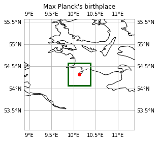
… that looks good ! Now we select the corresponding cells within the dark green window and display the indices.
Cells#
window_cell = (
    (grid.clat >= np.deg2rad(bottom_bound))
    & (grid.clat <= np.deg2rad(top_bound))
    & (grid.clon >= np.deg2rad(left_bound))
    & (grid.clon <= np.deg2rad(right_bound))
).values

(window_cell_indices,) = np.where(window_cell)
window_cell_indices
array([4282376, 4282377, 4282378, 4282400, 4282401, 4282402, 4282403,
       4282404, 4282405, 4282407, 4282408, 4282409, 4282410, 4282411,
       4282412, 4282413, 4282414, 4282415, 4282420, 4282421, 4282422,
       4282480, 4282481, 4282482, 4282483, 4282484, 4282485, 4282486,
       4282487, 4282488, 4282489, 4282490, 4282491, 4282493, 4282497,
       4282501, 4282508, 4282510, 4282511, 4282512, 4282513, 4282514,
       4282515, 4282516, 4282517, 4282518, 4282519, 4282520, 4282521,
       4282522, 4282523, 4282527, 4282558, 4282936, 4282938, 4282939,
       4282941, 4282960, 4282961, 4282962, 4282967, 4282968, 4282969,
       4282970, 4282971, 4282972, 4282973, 4283128, 4283129, 4283130])
What we have shown above are all the indices of the cells within the green window of the native grid. Since we selected them via np.where() we obtained the indices in 0-based python thinking. We now do the same for the vertices and edges that appear in our selected window:
Vertices#
We select with the function .isel() and the vertex_of_cell information from the grid all the vertices of the cells we have cut out one step before. We also sort the indices of the vertices and delete all duplicates vianp.unique(). Since the ICON code is written in Fortran, i.e. the integer-values are 1-based, we subtract 1 to get back to python thinking, hence 0-based.
window_vertex_indices = (
    np.unique(grid.vertex_of_cell.isel(cell=window_cell_indices).values) - 1
)
window_vertex_indices
array([2144929, 2144932, 2144933, 2144935, 2144937, 2144938, 2144939,
       2144953, 2144954, 2144955, 2144956, 2144957, 2144958, 2144959,
       2144960, 2144961, 2144962, 2144963, 2144968, 2144978, 2144983,
       2144984, 2145002, 2145003, 2145004, 2145005, 2145006, 2145007,
       2145008, 2145010, 2145011, 2145014, 2145020, 2145021, 2145022,
       2145023, 2145024, 2145025, 2145026, 2145217, 2145218, 2145220,
       2145222, 2145223, 2145224, 2145231, 2145237, 2145238, 2145239,
       2145286], dtype=int32)
Edges#
Same as for the vertices, we select with the function .isel() and the edge_of_cell information from the grid all the edges of the cells we have cut out two steps before. We also sort the indices of the edges and delete all duplicates via np.unique(). We subtract 1 to get back to python thinking.
window_edge_indices = (
    np.unique(grid.edge_of_cell.isel(cell=window_cell_indices).values) - 1
)
window_edge_indices
array([6427302, 6427311, 6427312, 6427313, 6427314, 6427315, 6427316,
       6427317, 6427318, 6427352, 6427353, 6427354, 6427355, 6427356,
       6427357, 6427358, 6427359, 6427360, 6427361, 6427362, 6427363,
       6427365, 6427366, 6427367, 6427368, 6427369, 6427370, 6427371,
       6427372, 6427373, 6427374, 6427375, 6427376, 6427377, 6427385,
       6427387, 6427388, 6427389, 6427390, 6427425, 6427426, 6427482,
       6427483, 6427484, 6427485, 6427486, 6427487, 6427488, 6427489,
       6427490, 6427491, 6427492, 6427493, 6427494, 6427495, 6427496,
       6427497, 6427498, 6427499, 6427500, 6427501, 6427504, 6427507,
       6427508, 6427513, 6427516, 6427527, 6427528, 6427529, 6427531,
       6427532, 6427533, 6427534, 6427535, 6427536, 6427537, 6427538,
       6427539, 6427540, 6427541, 6427542, 6427543, 6427544, 6427545,
       6427546, 6427547, 6427548, 6427549, 6427550, 6427553, 6427602,
       6428151, 6428152, 6428160, 6428161, 6428162, 6428164, 6428165,
       6428166, 6428167, 6428170, 6428202, 6428203, 6428204, 6428205,
       6428206, 6428207, 6428208, 6428213, 6428214, 6428215, 6428216,
       6428217, 6428218, 6428219, 6428410, 6428418, 6428419, 6428420],
      dtype=int32)
Constructing New Grid with Selected Cells, Vertices and Edges#
Wow, that’s already great ! We have received a lot of information in the form of indices in individual arrays about our green window. We merge them into one dataset so that everything is compact:
selected_indices = xr.Dataset(
    {
        "cell": ("cell", window_cell_indices),
        "vertex": ("vertex", window_vertex_indices),
        "edge": ("edge", window_edge_indices),
    }
)

selected_indices
<xarray.Dataset>
Dimensions:  (cell: 70, vertex: 50, edge: 119)
Coordinates:
  * cell     (cell) int64 4282376 4282377 4282378 ... 4283128 4283129 4283130
  * vertex   (vertex) int32 2144929 2144932 2144933 ... 2145238 2145239 2145286
  * edge     (edge) int32 6427302 6427311 6427312 ... 6428418 6428419 6428420
Data variables:
*empty*- cell: 70
- vertex: 50
- edge: 119
- cell(cell)int644282376 4282377 ... 4283129 4283130
array([4282376, 4282377, 4282378, 4282400, 4282401, 4282402, 4282403, 4282404, 4282405, 4282407, 4282408, 4282409, 4282410, 4282411, 4282412, 4282413, 4282414, 4282415, 4282420, 4282421, 4282422, 4282480, 4282481, 4282482, 4282483, 4282484, 4282485, 4282486, 4282487, 4282488, 4282489, 4282490, 4282491, 4282493, 4282497, 4282501, 4282508, 4282510, 4282511, 4282512, 4282513, 4282514, 4282515, 4282516, 4282517, 4282518, 4282519, 4282520, 4282521, 4282522, 4282523, 4282527, 4282558, 4282936, 4282938, 4282939, 4282941, 4282960, 4282961, 4282962, 4282967, 4282968, 4282969, 4282970, 4282971, 4282972, 4282973, 4283128, 4283129, 4283130]) - vertex(vertex)int322144929 2144932 ... 2145239 2145286
array([2144929, 2144932, 2144933, 2144935, 2144937, 2144938, 2144939, 2144953, 2144954, 2144955, 2144956, 2144957, 2144958, 2144959, 2144960, 2144961, 2144962, 2144963, 2144968, 2144978, 2144983, 2144984, 2145002, 2145003, 2145004, 2145005, 2145006, 2145007, 2145008, 2145010, 2145011, 2145014, 2145020, 2145021, 2145022, 2145023, 2145024, 2145025, 2145026, 2145217, 2145218, 2145220, 2145222, 2145223, 2145224, 2145231, 2145237, 2145238, 2145239, 2145286], dtype=int32) - edge(edge)int326427302 6427311 ... 6428419 6428420
array([6427302, 6427311, 6427312, 6427313, 6427314, 6427315, 6427316, 6427317,
       6427318, 6427352, 6427353, 6427354, 6427355, 6427356, 6427357, 6427358,
       6427359, 6427360, 6427361, 6427362, 6427363, 6427365, 6427366, 6427367,
       6427368, 6427369, 6427370, 6427371, 6427372, 6427373, 6427374, 6427375,
       6427376, 6427377, 6427385, 6427387, 6427388, 6427389, 6427390, 6427425,
       6427426, 6427482, 6427483, 6427484, 6427485, 6427486, 6427487, 6427488,
       6427489, 6427490, 6427491, 6427492, 6427493, 6427494, 6427495, 6427496,
       6427497, 6427498, 6427499, 6427500, 6427501, 6427504, 6427507, 6427508,
       6427513, 6427516, 6427527, 6427528, 6427529, 6427531, 6427532, 6427533,
       6427534, 6427535, 6427536, 6427537, 6427538, 6427539, 6427540, 6427541,
       6427542, 6427543, 6427544, 6427545, 6427546, 6427547, 6427548, 6427549,
       6427550, 6427553, 6427602, 6428151, 6428152, 6428160, 6428161, 6428162,
       6428164, 6428165, 6428166, 6428167, 6428170, 6428202, 6428203, 6428204,
       6428205, 6428206, 6428207, 6428208, 6428213, 6428214, 6428215, 6428216,
       6428217, 6428218, 6428219, 6428410, 6428418, 6428419, 6428420],
      dtype=int32)
It could be that we need more variables for future calculations. Therefore we create a dictionary with further interesting variables, which we reindex as a precaution.
vars_to_renumber = {
    "cell": [
        "adjacent_cell_of_edge",
        "cells_of_vertex",
        "neighbor_cell_index",
        "cell_index",
    ],
    "vertex": ["vertex_of_cell", "edge_vertices", "vertices_of_vertex"],
    "edge": ["edge_of_cell", "edges_of_vertex"],
}
We now come to the heart of this script: the reindexing.
Several things happen here, which is why it is best to define a function. This function reindex_grid() needs 3 inputs and returns 1 output. The inputs are the original, complete grid and the parts of the grid that should be reindexed, hence indices and vars_to_renumber. The indices define the cells, vertices and edges. The vars_to_renumber are all variables that we are still interested in and can be composed of cells, vertices and edges. Output of our function will be a new_grid containing all indices and variables for our green window around the birthplace of Max Planck in such a way that everything starts counting at 0.
Let’s go through it step by step:
Line 1: We define a function wiht 3 input variables.
Line 2: We define as new_grid the area in the old grid that contains the indices we selected at the beginning of this script for the cells, vertices and edges. For this we use the .load() function, which loads the 17GB file into memory and processes it there: this is a little faster.
Line 3: We open a for-loop that accesses the coordinates and the entries of the array selected_indices.
Line 4: We open an array, which is only filled with -2 (exceptional value like nan but as an integer) in the original, old grid length and call it renumbering.
Line 5: We start counting at 0 at the index positions of the long renumbering array, which belong to the indices of the selected dark green area, until we have reached the length of the short, previously selected array. So what we get is an array with the length of the original grid dimension (20971520 cells, 10485762 vertices, 31457280 edges), which contains a value other than -2 only at that position within the array which is inside the dark green selected window.
Line 6: we open another for loop over the remaining variables vars_to_renumber to be reindexed.
Line 7: For the variables stored in the dictionary of a particular dimension (cell, vertex, edge), we take one item and access it in new_grid (line 2) and subtract 1 to work in python 0-based system; this is done in the square brackets on the right side of the equal sign. We use this to select the valid position in the renumbering array but in total we add 1 to output the new_grid in the same 1-based thinking as the original grid.
Line 8: We output the new_grid.
def reindex_grid(grid, indices, vars_to_renumber):
    new_grid = grid.load().isel(
        cell=indices.cell, vertex=indices.vertex, edge=indices.edge
    )
    for dim, idx in indices.coords.items():
        renumbering = np.full(grid.dims[dim], -2, dtype="int")
        renumbering[idx] = np.arange(len(idx))
        for name in vars_to_renumber[dim]:
            new_grid[name].data = renumbering[new_grid[name].data - 1] + 1
    return new_grid
After long theory we want to use our function and create the actual new_grid:
new_grid = reindex_grid(grid, selected_indices, vars_to_renumber)
new_grid
<xarray.Dataset>
Dimensions:                         (cell: 70, nv: 3, vertex: 50, ne: 6,
                                     edge: 119, no: 4, nc: 2,
                                     max_stored_decompositions: 4, two_grf: 2,
                                     cell_grf: 14, max_chdom: 1, edge_grf: 24,
                                     vert_grf: 13)
Coordinates:
    clon                            (cell) float64 0.1804 0.1805 ... 0.174
    clat                            (cell) float64 0.9453 0.946 ... 0.9488
    vlon                            (vertex) float64 0.1815 0.1807 ... 0.1717
    vlat                            (vertex) float64 0.9456 0.9466 ... 0.9482
    elon                            (edge) float64 0.1811 0.1814 ... 0.1724
    elat                            (edge) float64 0.9461 0.9471 ... 0.9487
  * cell                            (cell) int64 4282376 4282377 ... 4283130
  * vertex                          (vertex) int32 2144929 2144932 ... 2145286
  * edge                            (edge) int32 6427302 6427311 ... 6428420
Dimensions without coordinates: nv, ne, no, nc, max_stored_decompositions,
                                two_grf, cell_grf, max_chdom, edge_grf, vert_grf
Data variables: (12/91)
    clon_vertices                   (cell, nv) float64 0.1794 0.1802 ... 0.173
    clat_vertices                   (cell, nv) float64 0.9457 0.9446 ... 0.9492
    vlon_vertices                   (vertex, ne) float64 9.969e+36 ... 9.969e+36
    vlat_vertices                   (vertex, ne) float64 9.969e+36 ... 9.969e+36
    elon_vertices                   (edge, no) float64 0.1807 0.1805 ... 0.1728
    elat_vertices                   (edge, no) float64 0.9466 0.946 ... 0.9485
    ...                              ...
    edge_dual_normal_cartesian_x    (edge) float64 -0.6706 -0.7373 ... -0.7362
    edge_dual_normal_cartesian_y    (edge) float64 -0.5071 0.4974 ... 0.4973
    edge_dual_normal_cartesian_z    (edge) float64 0.5414 0.4572 ... 0.4589
    cell_circumcenter_cartesian_x   (cell) float64 0.576 0.5755 ... 0.5739
    cell_circumcenter_cartesian_y   (cell) float64 0.105 0.105 ... 0.1003 0.1009
    cell_circumcenter_cartesian_z   (cell) float64 0.8107 0.8111 ... 0.8127
Attributes: (12/43)
    title:                    ICON grid description
    institution:              Max Planck Institute for Meteorology/Deutscher ...
    source:                   git@git.mpimet.mpg.de:GridGenerator.git
    revision:                 d00fcac1f61fa16c686bfe51d1d8eddd09296cb5
    date:                     20180529 at 222250
    user_name:                Rene Redler (m300083)
    ...                       ...
    topography:               modified SRTM30
    subcentre:                1
    number_of_grid_used:      15
    history:                  Thu Aug 16 11:05:44 2018: ncatted -O -a ICON_gr...
    ICON_grid_file_uri:       http://icon-downloads.mpimet.mpg.de/grids/publi...
NCO: netCDF Operators version 4.7.5 (Homepage = http...- cell: 70
- nv: 3
- vertex: 50
- ne: 6
- edge: 119
- no: 4
- nc: 2
- max_stored_decompositions: 4
- two_grf: 2
- cell_grf: 14
- max_chdom: 1
- edge_grf: 24
- vert_grf: 13
- clon(cell)float640.1804 0.1805 ... 0.1727 0.174
- long_name :
- center longitude
- units :
- radian
- standard_name :
- grid_longitude
- bounds :
- clon_vertices
array([0.18038067, 0.18050875, 0.17922247, 0.17886156, 0.17898882, 0.17770062, 0.1797501 , 0.18104121, 0.18091235, 0.18015244, 0.17693573, 0.17809803, 0.17604293, 0.17681007, 0.17846287, 0.17757454, 0.17833637, 0.17962243, 0.17997945, 0.18113629, 0.17909557, 0.17951792, 0.17862466, 0.17938988, 0.18068563, 0.17992138, 0.18081486, 0.18005019, 0.17875228, 0.17733185, 0.17745828, 0.17616818, 0.17822488, 0.18028089, 0.17385919, 0.17296933, 0.17589995, 0.17705416, 0.17501208, 0.17436905, 0.17552597, 0.17347672, 0.17424573, 0.17629139, 0.17513582, 0.17717949, 0.1764163 , 0.17475789, 0.17565046, 0.17488197, 0.17359962, 0.17309149, 0.17794004, 0.17321371, 0.1741108 , 0.17333694, 0.17256038, 0.17579145, 0.17462504, 0.17668901, 0.17372544, 0.17539795, 0.17450063, 0.17527312, 0.17656299, 0.17798397, 0.17785677, 0.17282752, 0.17270504, 0.17398714]) - clat(cell)float640.9453 0.946 ... 0.9478 0.9488
- long_name :
- center latitude
- units :
- radian
- standard_name :
- grid_latitude
- bounds :
- clat_vertices
array([0.9452853 , 0.94595806, 0.94500756, 0.94745215, 0.94812414, 0.94717332, 0.94704128, 0.94799093, 0.94731908, 0.94840249, 0.94825566, 0.94853505, 0.94866591, 0.94758354, 0.94609062, 0.94650081, 0.94541771, 0.9463689 , 0.94392414, 0.94420134, 0.94433427, 0.95015661, 0.95056824, 0.94948554, 0.95043502, 0.95151788, 0.95110557, 0.95218804, 0.95123892, 0.94961758, 0.95028879, 0.94933765, 0.94920664, 0.94907395, 0.94431485, 0.94472301, 0.94418628, 0.94446552, 0.9445951 , 0.94635069, 0.94663103, 0.94675957, 0.94567752, 0.94554846, 0.94526867, 0.94513895, 0.9462215 , 0.94771324, 0.94730368, 0.9483855 , 0.94743235, 0.94539671, 0.94405605, 0.94987657, 0.94946696, 0.95054805, 0.95162877, 0.95178156, 0.95150052, 0.95137057, 0.95191084, 0.95041926, 0.95082957, 0.94974792, 0.95069975, 0.95232086, 0.95165057, 0.94851365, 0.94784126, 0.94879509]) - vlon(vertex)float640.1815 0.1807 ... 0.1769 0.1717
- long_name :
- vertex longitude
- units :
- radian
- standard_name :
- grid_longitude
- bounds :
- vlon_vertices
array([0.18146698, 0.18071033, 0.18222101, 0.1820023 , 0.17942223, 0.18017984, 0.17813799, 0.17995105, 0.17789911, 0.17866199, 0.17918913, 0.17661297, 0.18124399, 0.17713357, 0.17584648, 0.17507733, 0.1773768 , 0.18093484, 0.17889655, 0.18178084, 0.18101821, 0.18025291, 0.17971943, 0.17842455, 0.18048304, 0.17765731, 0.17895315, 0.17636537, 0.17277765, 0.17481795, 0.17405225, 0.17200838, 0.17685758, 0.17609545, 0.17533068, 0.17456326, 0.17328389, 0.17251288, 0.17379317, 0.17224495, 0.17146679, 0.17353098, 0.1730204 , 0.1743055 , 0.17275375, 0.17818418, 0.17482091, 0.17559449, 0.17688738, 0.17173919]) - vlat(vertex)float640.9456 0.9466 ... 0.9521 0.9482
- long_name :
- vertex latitude
- units :
- radian
- standard_name :
- grid_latitude
- bounds :
- vlat_vertices
array([0.94555487, 0.94663854, 0.94447085, 0.94758786, 0.94568819, 0.94460468, 0.94473685, 0.94772185, 0.94785415, 0.94677135, 0.9488048 , 0.94690248, 0.94867133, 0.94893658, 0.94798476, 0.94906667, 0.94581984, 0.94352082, 0.94365349, 0.95070308, 0.951786 , 0.95286857, 0.95083721, 0.9498874 , 0.94975445, 0.95096964, 0.95191961, 0.95001866, 0.94404148, 0.94391382, 0.94499615, 0.94512328, 0.94378449, 0.94486733, 0.94594981, 0.94703193, 0.9460781 , 0.9471597 , 0.94811369, 0.95027609, 0.95135674, 0.95122941, 0.94919507, 0.95014823, 0.95231022, 0.95300165, 0.95218172, 0.95110038, 0.95205152, 0.94824092]) - elon(edge)float640.1811 0.1814 ... 0.1734 0.1724
- long_name :
- edge midpoint longitude
- units :
- radian
- standard_name :
- grid_longitude
- bounds :
- elon_vertices
array([0.18108894, 0.18135589, 0.1804447 , 0.17980132, 0.18082299, 0.18006586, 0.17877969, 0.17915901, 0.18120052, 0.17892518, 0.17828084, 0.1793061 , 0.17957038, 0.17854369, 0.17725561, 0.17763757, 0.18033098, 0.17968626, 0.18097677, 0.18162343, 0.18059709, 0.18021666, 0.17751663, 0.1764896 , 0.17687289, 0.17816145, 0.17610555, 0.1754622 , 0.17623001, 0.17801897, 0.17839961, 0.1790424 , 0.17699517, 0.17775768, 0.1815775 , 0.18055762, 0.17953777, 0.17991579, 0.17851755, 0.18063585, 0.18139982, 0.17907156, 0.17945389, 0.18010152, 0.17868846, 0.17804122, 0.17880713, 0.17983566, 0.18075023, 0.18113151, 0.18036839, 0.17998578, 0.17933658, 0.17960259, 0.17830479, 0.17739506, 0.17674976, 0.17777863, 0.17701091, 0.17572092, 0.1808638 , 0.17379789, 0.17341453, 0.17443538, 0.1723933 , 0.1730304 , 0.17583786, 0.1764768 , 0.17545628, 0.17749736, 0.17711681, 0.17507394, 0.17494726, 0.17392315, 0.17430738, 0.1759714 , 0.1755882 , 0.17353816, 0.17289868, 0.17469104, 0.17366836, 0.17571335, 0.1767357 , 0.17635383, 0.17520444, 0.17481992, 0.1741785 , 0.17443482, 0.1731526 , 0.17264571, 0.17787716, 0.17288753, 0.17249897, 0.17263297, 0.17366252, 0.17327532, 0.17404896, 0.17469171, 0.17391853, 0.17210984, 0.17314266, 0.17520799, 0.1762405 , 0.17585424, 0.17417551, 0.17456282, 0.17662599, 0.17727263, 0.17378742, 0.17494956, 0.17533553, 0.17598022, 0.17792036, 0.17856896, 0.17753535, 0.17212632, 0.17276627, 0.17340708, 0.17237937]) - elat(edge)float640.9461 0.9471 ... 0.9487 0.9487
- long_name :
- edge midpoint latitude
- units :
- radian
- standard_name :
- grid_latitude
- bounds :
- elat_vertices
array([0.94609674, 0.9471133 , 0.94562178, 0.94514647, 0.94507987, 0.94616346, 0.94521262, 0.94467101, 0.94453801, 0.94778825, 0.94731278, 0.9472467 , 0.94826336, 0.94832957, 0.94737841, 0.94683716, 0.94718023, 0.94670519, 0.9476551 , 0.94812963, 0.94819669, 0.94873832, 0.9483954 , 0.94846077, 0.9479197 , 0.94887094, 0.94900188, 0.94852575, 0.94744366, 0.94629569, 0.94575427, 0.94622981, 0.9463612 , 0.94527838, 0.94399593, 0.94406279, 0.94412919, 0.9435874 , 0.9441952 , 0.95232732, 0.95124458, 0.95036241, 0.94982118, 0.95029587, 0.95090368, 0.95042856, 0.94934614, 0.94927973, 0.9507704 , 0.95022887, 0.95131171, 0.95185306, 0.95137845, 0.95239419, 0.95144473, 0.94995328, 0.94947766, 0.94941209, 0.95049425, 0.94954277, 0.94921293, 0.9439779 , 0.94451891, 0.94445502, 0.94458242, 0.94505996, 0.9438494 , 0.94432595, 0.94439067, 0.94426077, 0.94480234, 0.94493199, 0.94649091, 0.94655511, 0.94601421, 0.94642624, 0.94696746, 0.94709606, 0.94661894, 0.94547308, 0.94553716, 0.94540861, 0.94534369, 0.94588508, 0.94750844, 0.94804947, 0.94757284, 0.94859028, 0.94763679, 0.94560079, 0.94371924, 0.95075285, 0.95129333, 0.94973562, 0.94967175, 0.95021241, 0.94913112, 0.94960749, 0.95068885, 0.95183358, 0.95176985, 0.95164109, 0.95157605, 0.95211687, 0.95170566, 0.95116514, 0.95103526, 0.95151062, 0.95224623, 0.9506244 , 0.95008369, 0.95055955, 0.95198582, 0.95246067, 0.95252669, 0.94770035, 0.94817755, 0.94865441, 0.9487181 ]) - cell(cell)int644282376 4282377 ... 4283129 4283130
array([4282376, 4282377, 4282378, 4282400, 4282401, 4282402, 4282403, 4282404, 4282405, 4282407, 4282408, 4282409, 4282410, 4282411, 4282412, 4282413, 4282414, 4282415, 4282420, 4282421, 4282422, 4282480, 4282481, 4282482, 4282483, 4282484, 4282485, 4282486, 4282487, 4282488, 4282489, 4282490, 4282491, 4282493, 4282497, 4282501, 4282508, 4282510, 4282511, 4282512, 4282513, 4282514, 4282515, 4282516, 4282517, 4282518, 4282519, 4282520, 4282521, 4282522, 4282523, 4282527, 4282558, 4282936, 4282938, 4282939, 4282941, 4282960, 4282961, 4282962, 4282967, 4282968, 4282969, 4282970, 4282971, 4282972, 4282973, 4283128, 4283129, 4283130]) - vertex(vertex)int322144929 2144932 ... 2145239 2145286
array([2144929, 2144932, 2144933, 2144935, 2144937, 2144938, 2144939, 2144953, 2144954, 2144955, 2144956, 2144957, 2144958, 2144959, 2144960, 2144961, 2144962, 2144963, 2144968, 2144978, 2144983, 2144984, 2145002, 2145003, 2145004, 2145005, 2145006, 2145007, 2145008, 2145010, 2145011, 2145014, 2145020, 2145021, 2145022, 2145023, 2145024, 2145025, 2145026, 2145217, 2145218, 2145220, 2145222, 2145223, 2145224, 2145231, 2145237, 2145238, 2145239, 2145286], dtype=int32) - edge(edge)int326427302 6427311 ... 6428419 6428420
array([6427302, 6427311, 6427312, 6427313, 6427314, 6427315, 6427316, 6427317,
       6427318, 6427352, 6427353, 6427354, 6427355, 6427356, 6427357, 6427358,
       6427359, 6427360, 6427361, 6427362, 6427363, 6427365, 6427366, 6427367,
       6427368, 6427369, 6427370, 6427371, 6427372, 6427373, 6427374, 6427375,
       6427376, 6427377, 6427385, 6427387, 6427388, 6427389, 6427390, 6427425,
       6427426, 6427482, 6427483, 6427484, 6427485, 6427486, 6427487, 6427488,
       6427489, 6427490, 6427491, 6427492, 6427493, 6427494, 6427495, 6427496,
       6427497, 6427498, 6427499, 6427500, 6427501, 6427504, 6427507, 6427508,
       6427513, 6427516, 6427527, 6427528, 6427529, 6427531, 6427532, 6427533,
       6427534, 6427535, 6427536, 6427537, 6427538, 6427539, 6427540, 6427541,
       6427542, 6427543, 6427544, 6427545, 6427546, 6427547, 6427548, 6427549,
       6427550, 6427553, 6427602, 6428151, 6428152, 6428160, 6428161, 6428162,
       6428164, 6428165, 6428166, 6428167, 6428170, 6428202, 6428203, 6428204,
       6428205, 6428206, 6428207, 6428208, 6428213, 6428214, 6428215, 6428216,
       6428217, 6428218, 6428219, 6428410, 6428418, 6428419, 6428420],
      dtype=int32)
- clon_vertices(cell, nv)float640.1794 0.1802 ... 0.1751 0.173
- units :
- radian
array([[0.17942223, 0.18017984, 0.18146698], [0.18146698, 0.18071033, 0.17942223], [0.17942223, 0.17813799, 0.18017984], [0.17995105, 0.17789911, 0.17866199], [0.17995105, 0.17918913, 0.17789911], [0.17789911, 0.17661297, 0.17866199], [0.17866199, 0.18071033, 0.17995105], [0.1820023 , 0.18124399, 0.17995105], [0.17995105, 0.18071033, 0.1820023 ], [0.18124399, 0.17918913, 0.17995105], [0.17713357, 0.17584648, 0.17789911], [0.17789911, 0.17918913, 0.17713357], [0.17713357, 0.17507733, 0.17584648], [0.17584648, 0.17661297, 0.17789911], [0.1773768 , 0.17942223, 0.17866199], [0.17866199, 0.17661297, 0.1773768 ], [0.1773768 , 0.17813799, 0.17942223], [0.17942223, 0.18071033, 0.17866199], [0.18017984, 0.17889655, 0.18093484], [0.18093484, 0.18222101, 0.18017984], ... [0.17379317, 0.17251288, 0.17456326], [0.17200838, 0.17405225, 0.17328389], [0.17889655, 0.17813799, 0.17685758], [0.1730204 , 0.1743055 , 0.17224495], [0.1730204 , 0.17507733, 0.1743055 ], [0.1743055 , 0.17353098, 0.17224495], [0.17146679, 0.17353098, 0.17275375], [0.17482091, 0.17559449, 0.17688738], [0.17482091, 0.17353098, 0.17559449], [0.17559449, 0.17765731, 0.17688738], [0.17275375, 0.17353098, 0.17482091], [0.1743055 , 0.17636537, 0.17559449], [0.17559449, 0.17353098, 0.1743055 ], [0.1743055 , 0.17507733, 0.17636537], [0.17636537, 0.17765731, 0.17559449], [0.17895315, 0.17818418, 0.17688738], [0.17688738, 0.17765731, 0.17895315], [0.17379317, 0.1730204 , 0.17173919], [0.17173919, 0.17251288, 0.17379317], [0.17379317, 0.17507733, 0.1730204 ]]) - clat_vertices(cell, nv)float640.9457 0.9446 ... 0.9491 0.9492
- units :
- radian
array([[0.94568819, 0.94460468, 0.94555487], [0.94555487, 0.94663854, 0.94568819], [0.94568819, 0.94473685, 0.94460468], [0.94772185, 0.94785415, 0.94677135], [0.94772185, 0.9488048 , 0.94785415], [0.94785415, 0.94690248, 0.94677135], [0.94677135, 0.94663854, 0.94772185], [0.94758786, 0.94867133, 0.94772185], [0.94772185, 0.94663854, 0.94758786], [0.94867133, 0.9488048 , 0.94772185], [0.94893658, 0.94798476, 0.94785415], [0.94785415, 0.9488048 , 0.94893658], [0.94893658, 0.94906667, 0.94798476], [0.94798476, 0.94690248, 0.94785415], [0.94581984, 0.94568819, 0.94677135], [0.94677135, 0.94690248, 0.94581984], [0.94581984, 0.94473685, 0.94568819], [0.94568819, 0.94663854, 0.94677135], [0.94460468, 0.94365349, 0.94352082], [0.94352082, 0.94447085, 0.94460468], ... [0.94811369, 0.9471597 , 0.94703193], [0.94512328, 0.94499615, 0.9460781 ], [0.94365349, 0.94473685, 0.94378449], [0.94919507, 0.95014823, 0.95027609], [0.94919507, 0.94906667, 0.95014823], [0.95014823, 0.95122941, 0.95027609], [0.95135674, 0.95122941, 0.95231022], [0.95218172, 0.95110038, 0.95205152], [0.95218172, 0.95122941, 0.95110038], [0.95110038, 0.95096964, 0.95205152], [0.95231022, 0.95122941, 0.95218172], [0.95014823, 0.95001866, 0.95110038], [0.95110038, 0.95122941, 0.95014823], [0.95014823, 0.94906667, 0.95001866], [0.95001866, 0.95096964, 0.95110038], [0.95191961, 0.95300165, 0.95205152], [0.95205152, 0.95096964, 0.95191961], [0.94811369, 0.94919507, 0.94824092], [0.94824092, 0.9471597 , 0.94811369], [0.94811369, 0.94906667, 0.94919507]]) - vlon_vertices(vertex, ne)float649.969e+36 9.969e+36 ... 9.969e+36
- units :
- radian
array([[9.96920997e+36, 9.96920997e+36, 9.96920997e+36, 9.96920997e+36, 9.96920997e+36, 9.96920997e+36], [9.96920997e+36, 9.96920997e+36, 9.96920997e+36, 9.96920997e+36, 9.96920997e+36, 9.96920997e+36], [9.96920997e+36, 9.96920997e+36, 9.96920997e+36, 9.96920997e+36, 9.96920997e+36, 9.96920997e+36], [9.96920997e+36, 9.96920997e+36, 9.96920997e+36, 9.96920997e+36, 9.96920997e+36, 9.96920997e+36], [9.96920997e+36, 9.96920997e+36, 9.96920997e+36, 9.96920997e+36, 9.96920997e+36, 9.96920997e+36], [9.96920997e+36, 9.96920997e+36, 9.96920997e+36, 9.96920997e+36, 9.96920997e+36, 9.96920997e+36], [9.96920997e+36, 9.96920997e+36, 9.96920997e+36, 9.96920997e+36, 9.96920997e+36, 9.96920997e+36], [9.96920997e+36, 9.96920997e+36, 9.96920997e+36, 9.96920997e+36, 9.96920997e+36, 9.96920997e+36], [9.96920997e+36, 9.96920997e+36, 9.96920997e+36, 9.96920997e+36, 9.96920997e+36, 9.96920997e+36], [9.96920997e+36, 9.96920997e+36, 9.96920997e+36, 9.96920997e+36, 9.96920997e+36, 9.96920997e+36], ... [9.96920997e+36, 9.96920997e+36, 9.96920997e+36, 9.96920997e+36, 9.96920997e+36, 9.96920997e+36], [9.96920997e+36, 9.96920997e+36, 9.96920997e+36, 9.96920997e+36, 9.96920997e+36, 9.96920997e+36], [9.96920997e+36, 9.96920997e+36, 9.96920997e+36, 9.96920997e+36, 9.96920997e+36, 9.96920997e+36], [9.96920997e+36, 9.96920997e+36, 9.96920997e+36, 9.96920997e+36, 9.96920997e+36, 9.96920997e+36], [9.96920997e+36, 9.96920997e+36, 9.96920997e+36, 9.96920997e+36, 9.96920997e+36, 9.96920997e+36], [9.96920997e+36, 9.96920997e+36, 9.96920997e+36, 9.96920997e+36, 9.96920997e+36, 9.96920997e+36], [9.96920997e+36, 9.96920997e+36, 9.96920997e+36, 9.96920997e+36, 9.96920997e+36, 9.96920997e+36], [9.96920997e+36, 9.96920997e+36, 9.96920997e+36, 9.96920997e+36, 9.96920997e+36, 9.96920997e+36], [9.96920997e+36, 9.96920997e+36, 9.96920997e+36, 9.96920997e+36, 9.96920997e+36, 9.96920997e+36], [9.96920997e+36, 9.96920997e+36, 9.96920997e+36, 9.96920997e+36, 9.96920997e+36, 9.96920997e+36]]) - vlat_vertices(vertex, ne)float649.969e+36 9.969e+36 ... 9.969e+36
- units :
- radian
array([[9.96920997e+36, 9.96920997e+36, 9.96920997e+36, 9.96920997e+36, 9.96920997e+36, 9.96920997e+36], [9.96920997e+36, 9.96920997e+36, 9.96920997e+36, 9.96920997e+36, 9.96920997e+36, 9.96920997e+36], [9.96920997e+36, 9.96920997e+36, 9.96920997e+36, 9.96920997e+36, 9.96920997e+36, 9.96920997e+36], [9.96920997e+36, 9.96920997e+36, 9.96920997e+36, 9.96920997e+36, 9.96920997e+36, 9.96920997e+36], [9.96920997e+36, 9.96920997e+36, 9.96920997e+36, 9.96920997e+36, 9.96920997e+36, 9.96920997e+36], [9.96920997e+36, 9.96920997e+36, 9.96920997e+36, 9.96920997e+36, 9.96920997e+36, 9.96920997e+36], [9.96920997e+36, 9.96920997e+36, 9.96920997e+36, 9.96920997e+36, 9.96920997e+36, 9.96920997e+36], [9.96920997e+36, 9.96920997e+36, 9.96920997e+36, 9.96920997e+36, 9.96920997e+36, 9.96920997e+36], [9.96920997e+36, 9.96920997e+36, 9.96920997e+36, 9.96920997e+36, 9.96920997e+36, 9.96920997e+36], [9.96920997e+36, 9.96920997e+36, 9.96920997e+36, 9.96920997e+36, 9.96920997e+36, 9.96920997e+36], ... [9.96920997e+36, 9.96920997e+36, 9.96920997e+36, 9.96920997e+36, 9.96920997e+36, 9.96920997e+36], [9.96920997e+36, 9.96920997e+36, 9.96920997e+36, 9.96920997e+36, 9.96920997e+36, 9.96920997e+36], [9.96920997e+36, 9.96920997e+36, 9.96920997e+36, 9.96920997e+36, 9.96920997e+36, 9.96920997e+36], [9.96920997e+36, 9.96920997e+36, 9.96920997e+36, 9.96920997e+36, 9.96920997e+36, 9.96920997e+36], [9.96920997e+36, 9.96920997e+36, 9.96920997e+36, 9.96920997e+36, 9.96920997e+36, 9.96920997e+36], [9.96920997e+36, 9.96920997e+36, 9.96920997e+36, 9.96920997e+36, 9.96920997e+36, 9.96920997e+36], [9.96920997e+36, 9.96920997e+36, 9.96920997e+36, 9.96920997e+36, 9.96920997e+36, 9.96920997e+36], [9.96920997e+36, 9.96920997e+36, 9.96920997e+36, 9.96920997e+36, 9.96920997e+36, 9.96920997e+36], [9.96920997e+36, 9.96920997e+36, 9.96920997e+36, 9.96920997e+36, 9.96920997e+36, 9.96920997e+36], [9.96920997e+36, 9.96920997e+36, 9.96920997e+36, 9.96920997e+36, 9.96920997e+36, 9.96920997e+36]]) - elon_vertices(edge, no)float640.1807 0.1805 ... 0.1717 0.1728
- units :
- radian
array([[0.18071033, 0.18050875, 0.18146698, 0.18166963], [0.1820023 , 0.18091235, 0.18071033, 0.18179889], [0.18146698, 0.18050875, 0.17942223, 0.18038067], [0.17942223, 0.17922247, 0.18017984, 0.18038067], [0.18017984, 0.18126477, 0.18146698, 0.18038067], [0.18071033, 0.17962243, 0.17942223, 0.18050875], [0.17942223, 0.17833637, 0.17813799, 0.17922247], [0.17813799, 0.17909557, 0.18017984, 0.17922247], [0.18017984, 0.18113629, 0.18222101, 0.18126477], [0.17995105, 0.17898882, 0.17789911, 0.17886156], [0.17789911, 0.17770062, 0.17866199, 0.17886156], [0.17866199, 0.1797501 , 0.17995105, 0.17886156], [0.17995105, 0.18015244, 0.17918913, 0.17898882], [0.17918913, 0.17809803, 0.17789911, 0.17898882], [0.17789911, 0.17681007, 0.17661297, 0.17770062], [0.17661297, 0.17757454, 0.17866199, 0.17770062], [0.18071033, 0.18091235, 0.17995105, 0.1797501 ], [0.17866199, 0.17962243, 0.18071033, 0.1797501 ], [0.17995105, 0.18091235, 0.1820023 , 0.18104121], [0.1820023 , 0.18220615, 0.18124399, 0.18104121], ... [0.17146679, 0.17256038, 0.17275375, 0.17165875], [0.17353098, 0.17372544, 0.17275375, 0.17256038], [0.17482091, 0.17462504, 0.17559449, 0.17579145], [0.17559449, 0.17668901, 0.17688738, 0.17579145], [0.17688738, 0.17591704, 0.17482091, 0.17579145], [0.17482091, 0.17372544, 0.17353098, 0.17462504], [0.17353098, 0.17450063, 0.17559449, 0.17462504], [0.17559449, 0.17656299, 0.17765731, 0.17668901], [0.17765731, 0.17785677, 0.17688738, 0.17668901], [0.17275375, 0.17372544, 0.17482091, 0.17384942], [0.17559449, 0.17450063, 0.1743055 , 0.17539795], [0.1743055 , 0.17527312, 0.17636537, 0.17539795], [0.17636537, 0.17656299, 0.17559449, 0.17539795], [0.17688738, 0.17785677, 0.17895315, 0.17798397], [0.17895315, 0.17915446, 0.17818418, 0.17798397], [0.17818418, 0.17708618, 0.17688738, 0.17798397], [0.17251288, 0.17270504, 0.17173919, 0.17154812], [0.17173919, 0.17270504, 0.17379317, 0.17282752], [0.17379317, 0.17398714, 0.1730204 , 0.17282752], [0.1730204 , 0.17193068, 0.17173919, 0.17282752]]) - elat_vertices(edge, no)float640.9466 0.946 ... 0.9482 0.9485
- units :
- radian
array([[0.94663854, 0.94595806, 0.94555487, 0.94623532], [0.94758786, 0.94731908, 0.94663854, 0.94690755], [0.94555487, 0.94595806, 0.94568819, 0.9452853 ], [0.94568819, 0.94500756, 0.94460468, 0.9452853 ], [0.94460468, 0.94487449, 0.94555487, 0.9452853 ], [0.94663854, 0.9463689 , 0.94568819, 0.94595806], [0.94568819, 0.94541771, 0.94473685, 0.94500756], [0.94473685, 0.94433427, 0.94460468, 0.94500756], [0.94460468, 0.94420134, 0.94447085, 0.94487449], [0.94772185, 0.94812414, 0.94785415, 0.94745215], [0.94785415, 0.94717332, 0.94677135, 0.94745215], [0.94677135, 0.94704128, 0.94772185, 0.94745215], [0.94772185, 0.94840249, 0.9488048 , 0.94812414], [0.9488048 , 0.94853505, 0.94785415, 0.94812414], [0.94785415, 0.94758354, 0.94690248, 0.94717332], [0.94690248, 0.94650081, 0.94677135, 0.94717332], [0.94663854, 0.94731908, 0.94772185, 0.94704128], [0.94677135, 0.9463689 , 0.94663854, 0.94704128], [0.94772185, 0.94731908, 0.94758786, 0.94799093], [0.94758786, 0.94826824, 0.94867133, 0.94799093], ... [0.95135674, 0.95162877, 0.95231022, 0.95203843], [0.95122941, 0.95191084, 0.95231022, 0.95162877], [0.95218172, 0.95150052, 0.95110038, 0.95178156], [0.95110038, 0.95137057, 0.95205152, 0.95178156], [0.95205152, 0.95245199, 0.95218172, 0.95178156], [0.95218172, 0.95191084, 0.95122941, 0.95150052], [0.95122941, 0.95082957, 0.95110038, 0.95150052], [0.95110038, 0.95069975, 0.95096964, 0.95137057], [0.95096964, 0.95165057, 0.95205152, 0.95137057], [0.95231022, 0.95191084, 0.95218172, 0.95258141], [0.95110038, 0.95082957, 0.95014823, 0.95041926], [0.95014823, 0.94974792, 0.95001866, 0.95041926], [0.95001866, 0.95069975, 0.95110038, 0.95041926], [0.95205152, 0.95165057, 0.95191961, 0.95232086], [0.95191961, 0.95260038, 0.95300165, 0.95232086], [0.95300165, 0.95273254, 0.95205152, 0.95232086], [0.9471597 , 0.94784126, 0.94824092, 0.94755934], [0.94824092, 0.94784126, 0.94811369, 0.94851365], [0.94811369, 0.94879509, 0.94919507, 0.94851365], [0.94919507, 0.94892258, 0.94824092, 0.94851365]]) - ifs2icon_cell_grid(cell)float649.969e+36 9.969e+36 ... 9.969e+36
- long_name :
- ifs to icon cells
array([9.96920997e+36, 9.96920997e+36, 9.96920997e+36, 9.96920997e+36, 9.96920997e+36, 9.96920997e+36, 9.96920997e+36, 9.96920997e+36, 9.96920997e+36, 9.96920997e+36, 9.96920997e+36, 9.96920997e+36, 9.96920997e+36, 9.96920997e+36, 9.96920997e+36, 9.96920997e+36, 9.96920997e+36, 9.96920997e+36, 9.96920997e+36, 9.96920997e+36, 9.96920997e+36, 9.96920997e+36, 9.96920997e+36, 9.96920997e+36, 9.96920997e+36, 9.96920997e+36, 9.96920997e+36, 9.96920997e+36, 9.96920997e+36, 9.96920997e+36, 9.96920997e+36, 9.96920997e+36, 9.96920997e+36, 9.96920997e+36, 9.96920997e+36, 9.96920997e+36, 9.96920997e+36, 9.96920997e+36, 9.96920997e+36, 9.96920997e+36, 9.96920997e+36, 9.96920997e+36, 9.96920997e+36, 9.96920997e+36, 9.96920997e+36, 9.96920997e+36, 9.96920997e+36, 9.96920997e+36, 9.96920997e+36, 9.96920997e+36, 9.96920997e+36, 9.96920997e+36, 9.96920997e+36, 9.96920997e+36, 9.96920997e+36, 9.96920997e+36, 9.96920997e+36, 9.96920997e+36, 9.96920997e+36, 9.96920997e+36, 9.96920997e+36, 9.96920997e+36, 9.96920997e+36, 9.96920997e+36, 9.96920997e+36, 9.96920997e+36, 9.96920997e+36, 9.96920997e+36, 9.96920997e+36, 9.96920997e+36]) - ifs2icon_edge_grid(edge)float649.969e+36 9.969e+36 ... 9.969e+36
- long_name :
- ifs to icon edge
array([9.96920997e+36, 9.96920997e+36, 9.96920997e+36, 9.96920997e+36, 9.96920997e+36, 9.96920997e+36, 9.96920997e+36, 9.96920997e+36, 9.96920997e+36, 9.96920997e+36, 9.96920997e+36, 9.96920997e+36, 9.96920997e+36, 9.96920997e+36, 9.96920997e+36, 9.96920997e+36, 9.96920997e+36, 9.96920997e+36, 9.96920997e+36, 9.96920997e+36, 9.96920997e+36, 9.96920997e+36, 9.96920997e+36, 9.96920997e+36, 9.96920997e+36, 9.96920997e+36, 9.96920997e+36, 9.96920997e+36, 9.96920997e+36, 9.96920997e+36, 9.96920997e+36, 9.96920997e+36, 9.96920997e+36, 9.96920997e+36, 9.96920997e+36, 9.96920997e+36, 9.96920997e+36, 9.96920997e+36, 9.96920997e+36, 9.96920997e+36, 9.96920997e+36, 9.96920997e+36, 9.96920997e+36, 9.96920997e+36, 9.96920997e+36, 9.96920997e+36, 9.96920997e+36, 9.96920997e+36, 9.96920997e+36, 9.96920997e+36, 9.96920997e+36, 9.96920997e+36, 9.96920997e+36, 9.96920997e+36, 9.96920997e+36, 9.96920997e+36, 9.96920997e+36, 9.96920997e+36, 9.96920997e+36, 9.96920997e+36, 9.96920997e+36, 9.96920997e+36, 9.96920997e+36, 9.96920997e+36, 9.96920997e+36, 9.96920997e+36, 9.96920997e+36, 9.96920997e+36, 9.96920997e+36, 9.96920997e+36, 9.96920997e+36, 9.96920997e+36, 9.96920997e+36, 9.96920997e+36, 9.96920997e+36, 9.96920997e+36, 9.96920997e+36, 9.96920997e+36, 9.96920997e+36, 9.96920997e+36, 9.96920997e+36, 9.96920997e+36, 9.96920997e+36, 9.96920997e+36, 9.96920997e+36, 9.96920997e+36, 9.96920997e+36, 9.96920997e+36, 9.96920997e+36, 9.96920997e+36, 9.96920997e+36, 9.96920997e+36, 9.96920997e+36, 9.96920997e+36, 9.96920997e+36, 9.96920997e+36, 9.96920997e+36, 9.96920997e+36, 9.96920997e+36, 9.96920997e+36, 9.96920997e+36, 9.96920997e+36, 9.96920997e+36, 9.96920997e+36, 9.96920997e+36, 9.96920997e+36, 9.96920997e+36, 9.96920997e+36, 9.96920997e+36, 9.96920997e+36, 9.96920997e+36, 9.96920997e+36, 9.96920997e+36, 9.96920997e+36, 9.96920997e+36, 9.96920997e+36, 9.96920997e+36, 9.96920997e+36, 9.96920997e+36]) - ifs2icon_vertex_grid(vertex)float649.969e+36 9.969e+36 ... 9.969e+36
- long_name :
- ifs to icon vertex
array([9.96920997e+36, 9.96920997e+36, 9.96920997e+36, 9.96920997e+36, 9.96920997e+36, 9.96920997e+36, 9.96920997e+36, 9.96920997e+36, 9.96920997e+36, 9.96920997e+36, 9.96920997e+36, 9.96920997e+36, 9.96920997e+36, 9.96920997e+36, 9.96920997e+36, 9.96920997e+36, 9.96920997e+36, 9.96920997e+36, 9.96920997e+36, 9.96920997e+36, 9.96920997e+36, 9.96920997e+36, 9.96920997e+36, 9.96920997e+36, 9.96920997e+36, 9.96920997e+36, 9.96920997e+36, 9.96920997e+36, 9.96920997e+36, 9.96920997e+36, 9.96920997e+36, 9.96920997e+36, 9.96920997e+36, 9.96920997e+36, 9.96920997e+36, 9.96920997e+36, 9.96920997e+36, 9.96920997e+36, 9.96920997e+36, 9.96920997e+36, 9.96920997e+36, 9.96920997e+36, 9.96920997e+36, 9.96920997e+36, 9.96920997e+36, 9.96920997e+36, 9.96920997e+36, 9.96920997e+36, 9.96920997e+36, 9.96920997e+36]) - cell_area(cell)float642.512e+07 2.512e+07 ... 2.513e+07
- long_name :
- area of grid cell
- units :
- m2
- standard_name :
- area
- grid_type :
- unstructured
- number_of_grid_in_reference :
- 1
array([25122696.10073513, 25115307.26790699, 25116300.53412801, 25123237.93102442, 25115830.24743506, 25116842.75658992, 25115578.91013796, 25114562.04009542, 25121960.93224146, 25122212.05939919, 25117083.44892931, 25123478.41462998, 25124729.65854212, 25124499.79352248, 25116581.78490075, 25124249.66579937, 25123979.27550808, 25122977.15964761, 25115999.00466688, 25122394.75463809, 25123688.62295523, 25115025.06352181, 25122653.37508515, 25122442.87366889, 25121393.21509447, 25121593.99702691, 25113974.84572285, 25114166.12429192, 25115226.07920017, 25123698.61042375, 25116272.0067958 , 25117303.86182249, 25116061.27965469, 25114803.71718214, 25119795.71590116, 25127478.52325461, 25118545.37157181, 25124967.23612089, 25126230.55054701, 25119085.46937051, 25125506.96657332, 25126749.0184048 , 25126499.89063621, 25125247.21999242, 25118825.53430106, 25117570.61997183, 25117841.20015365, 25125746.47559248, 25118091.526784 , 25118321.59969451, 25119325.17646931, 25120065.2334573 , 25117279.78659467, 25126164.78076905, 25118531.41881819, 25118720.98430478, 25118890.29643543, 25124078.13911133, 25117683.8497022 , 25116462.42901175, 25125297.67809606, 25117503.99534079, 25125128.60058216, 25124939.26083178, 25123898.51849904, 25115406.76447713, 25122843.56384486, 25119544.65546474, 25126977.93366472, 25125965.74696781]) - dual_area(vertex)float645.024e+07 5.024e+07 ... 5.025e+07
- long_name :
- areas of dual hexagonal/pentagonal cells
- units :
- m2
- standard_name :
- area
array([50236704.12265563, 50237267.52765939, 50236100.11867585, 50235230.03800005, 50239276.96625393, 50238694.37788524, 50241258.30509415, 50237790.28838633, 50240320.46429419, 50239819.00547045, 50238272.44700849, 50242340.25239363, 50235733.50250239, 50240781.35013165, 50242820.45288354, 50243260.11567578, 50241819.53384106, 50238071.21177694, 50240656.57054461, 50234092.08434241, 50234494.79437514, 50234856.73413058, 50236618.42800296, 50238714.00341169, 50236196.29512241, 50239114.91664437, 50236999.90949156, 50241201.68542749, 50248229.36952424, 50245735.70412067, 50246294.79118221, 50248767.16638389, 50243211.42616763, 50243791.78421131, 50244331.72451836, 50244831.15801625, 50246813.43715227, 50247291.67618234, 50245290.15457646, 50246086.7301536 , 50246424.31658242, 50244017.9306002 , 50245708.66943013, 50243659.30219435, 50244336.07246792, 50237340.69553816, 50241920.64027966, 50241581.43129943, 50239475.19993137, 50247729.49309564]) - phys_cell_id(cell)int321 1 1 1 1 1 1 1 ... 1 1 1 1 1 1 1 1
- long_name :
- physical domain ID of cell
- grid_type :
- unstructured
- number_of_grid_in_reference :
- 1
array([1, 1, 1, 1, 1, 1, 1, 1, 1, 1, 1, 1, 1, 1, 1, 1, 1, 1, 1, 1, 1, 1, 1, 1, 1, 1, 1, 1, 1, 1, 1, 1, 1, 1, 1, 1, 1, 1, 1, 1, 1, 1, 1, 1, 1, 1, 1, 1, 1, 1, 1, 1, 1, 1, 1, 1, 1, 1, 1, 1, 1, 1, 1, 1, 1, 1, 1, 1, 1, 1], dtype=int32) - phys_edge_id(edge)int321 1 1 1 1 1 1 1 ... 1 1 1 1 1 1 1 1
- long_name :
- physical domain ID of edge
array([1, 1, 1, 1, 1, 1, 1, 1, 1, 1, 1, 1, 1, 1, 1, 1, 1, 1, 1, 1, 1, 1, 1, 1, 1, 1, 1, 1, 1, 1, 1, 1, 1, 1, 1, 1, 1, 1, 1, 1, 1, 1, 1, 1, 1, 1, 1, 1, 1, 1, 1, 1, 1, 1, 1, 1, 1, 1, 1, 1, 1, 1, 1, 1, 1, 1, 1, 1, 1, 1, 1, 1, 1, 1, 1, 1, 1, 1, 1, 1, 1, 1, 1, 1, 1, 1, 1, 1, 1, 1, 1, 1, 1, 1, 1, 1, 1, 1, 1, 1, 1, 1, 1, 1, 1, 1, 1, 1, 1, 1, 1, 1, 1, 1, 1, 1, 1, 1, 1], dtype=int32) - lon_cell_centre(cell)float640.1804 0.1805 ... 0.1727 0.174
- long_name :
- longitude of cell centre
- units :
- radian
- grid_type :
- unstructured
- number_of_grid_in_reference :
- 1
array([0.18038067, 0.18050875, 0.17922247, 0.17886156, 0.17898882, 0.17770062, 0.1797501 , 0.18104121, 0.18091235, 0.18015244, 0.17693573, 0.17809803, 0.17604293, 0.17681007, 0.17846287, 0.17757454, 0.17833637, 0.17962243, 0.17997945, 0.18113629, 0.17909557, 0.17951792, 0.17862466, 0.17938988, 0.18068563, 0.17992138, 0.18081486, 0.18005019, 0.17875228, 0.17733185, 0.17745828, 0.17616818, 0.17822488, 0.18028089, 0.17385919, 0.17296933, 0.17589995, 0.17705416, 0.17501208, 0.17436905, 0.17552597, 0.17347672, 0.17424573, 0.17629139, 0.17513582, 0.17717949, 0.1764163 , 0.17475789, 0.17565046, 0.17488197, 0.17359962, 0.17309149, 0.17794004, 0.17321371, 0.1741108 , 0.17333694, 0.17256038, 0.17579145, 0.17462504, 0.17668901, 0.17372544, 0.17539795, 0.17450063, 0.17527312, 0.17656299, 0.17798397, 0.17785677, 0.17282752, 0.17270504, 0.17398714]) - lat_cell_centre(cell)float640.9453 0.946 ... 0.9478 0.9488
- long_name :
- latitude of cell centre
- units :
- radian
- grid_type :
- unstructured
- number_of_grid_in_reference :
- 1
array([0.9452853 , 0.94595806, 0.94500756, 0.94745215, 0.94812414, 0.94717332, 0.94704128, 0.94799093, 0.94731908, 0.94840249, 0.94825566, 0.94853505, 0.94866591, 0.94758354, 0.94609062, 0.94650081, 0.94541771, 0.9463689 , 0.94392414, 0.94420134, 0.94433427, 0.95015661, 0.95056824, 0.94948554, 0.95043502, 0.95151788, 0.95110557, 0.95218804, 0.95123892, 0.94961758, 0.95028879, 0.94933765, 0.94920664, 0.94907395, 0.94431485, 0.94472301, 0.94418628, 0.94446552, 0.9445951 , 0.94635069, 0.94663103, 0.94675957, 0.94567752, 0.94554846, 0.94526867, 0.94513895, 0.9462215 , 0.94771324, 0.94730368, 0.9483855 , 0.94743235, 0.94539671, 0.94405605, 0.94987657, 0.94946696, 0.95054805, 0.95162877, 0.95178156, 0.95150052, 0.95137057, 0.95191084, 0.95041926, 0.95082957, 0.94974792, 0.95069975, 0.95232086, 0.95165057, 0.94851365, 0.94784126, 0.94879509]) - lat_cell_barycenter(cell)float640.9453 0.946 ... 0.9478 0.9488
- long_name :
- latitude of cell barycenter
- units :
- radian
- grid_type :
- unstructured
- number_of_grid_in_reference :
- 1
array([0.94528275, 0.9459607 , 0.94501008, 0.94744928, 0.9481271 , 0.94717616, 0.94704408, 0.94799385, 0.94731625, 0.9483995 , 0.94825867, 0.94853202, 0.94866284, 0.94758063, 0.9460933 , 0.94649806, 0.94541513, 0.9463662 , 0.9439265 , 0.94419895, 0.94433184, 0.95015986, 0.95056492, 0.94948239, 0.95043175, 0.95151445, 0.95110894, 0.95219157, 0.95124233, 0.94961439, 0.95029207, 0.94934081, 0.94920977, 0.94907703, 0.94431732, 0.94472047, 0.94418872, 0.94446306, 0.9445926 , 0.94635345, 0.94662824, 0.94675675, 0.94567486, 0.94554583, 0.94527127, 0.94514151, 0.94622421, 0.9477103 , 0.94730656, 0.94838854, 0.94743527, 0.94539935, 0.94405845, 0.9498733 , 0.94947016, 0.95055141, 0.9516323 , 0.95177804, 0.95150401, 0.95137402, 0.95190729, 0.95042259, 0.95082617, 0.94974469, 0.9506964 , 0.95232443, 0.9516471 , 0.94851673, 0.94783827, 0.94879198]) - lon_cell_barycenter(cell)float640.1804 0.1805 ... 0.1727 0.174
- long_name :
- longitude of cell barycenter
- units :
- radian
- grid_type :
- unstructured
- number_of_grid_in_reference :
- 1
array([0.18035633, 0.18053316, 0.17924667, 0.17883737, 0.17901308, 0.17772467, 0.17977444, 0.18106576, 0.18088787, 0.18012804, 0.1769597 , 0.17807392, 0.17601911, 0.17678617, 0.17848699, 0.17755057, 0.17831232, 0.17959817, 0.18000372, 0.18111188, 0.17907144, 0.17954232, 0.17860041, 0.17936555, 0.18066108, 0.17989691, 0.18083947, 0.18007474, 0.17877661, 0.17730781, 0.17748239, 0.17619207, 0.17824907, 0.18030537, 0.17388259, 0.17294607, 0.17592364, 0.17703032, 0.17498853, 0.17439259, 0.17550228, 0.17345332, 0.17422225, 0.17626762, 0.17515944, 0.17720339, 0.17644013, 0.17473428, 0.17567422, 0.17490564, 0.17362308, 0.17311482, 0.17796402, 0.17319026, 0.17413439, 0.17336046, 0.17258382, 0.17576757, 0.17464877, 0.17671304, 0.17370186, 0.17542177, 0.17447697, 0.17524938, 0.17653903, 0.17800822, 0.17783259, 0.1728509 , 0.17268173, 0.17396362]) - longitude_vertices(vertex)float640.1815 0.1807 ... 0.1769 0.1717
- long_name :
- longitude of vertices
- units :
- radian
array([0.18146698, 0.18071033, 0.18222101, 0.1820023 , 0.17942223, 0.18017984, 0.17813799, 0.17995105, 0.17789911, 0.17866199, 0.17918913, 0.17661297, 0.18124399, 0.17713357, 0.17584648, 0.17507733, 0.1773768 , 0.18093484, 0.17889655, 0.18178084, 0.18101821, 0.18025291, 0.17971943, 0.17842455, 0.18048304, 0.17765731, 0.17895315, 0.17636537, 0.17277765, 0.17481795, 0.17405225, 0.17200838, 0.17685758, 0.17609545, 0.17533068, 0.17456326, 0.17328389, 0.17251288, 0.17379317, 0.17224495, 0.17146679, 0.17353098, 0.1730204 , 0.1743055 , 0.17275375, 0.17818418, 0.17482091, 0.17559449, 0.17688738, 0.17173919]) - latitude_vertices(vertex)float640.9456 0.9466 ... 0.9521 0.9482
- long_name :
- latitude of vertices
- units :
- radian
array([0.94555487, 0.94663854, 0.94447085, 0.94758786, 0.94568819, 0.94460468, 0.94473685, 0.94772185, 0.94785415, 0.94677135, 0.9488048 , 0.94690248, 0.94867133, 0.94893658, 0.94798476, 0.94906667, 0.94581984, 0.94352082, 0.94365349, 0.95070308, 0.951786 , 0.95286857, 0.95083721, 0.9498874 , 0.94975445, 0.95096964, 0.95191961, 0.95001866, 0.94404148, 0.94391382, 0.94499615, 0.94512328, 0.94378449, 0.94486733, 0.94594981, 0.94703193, 0.9460781 , 0.9471597 , 0.94811369, 0.95027609, 0.95135674, 0.95122941, 0.94919507, 0.95014823, 0.95231022, 0.95300165, 0.95218172, 0.95110038, 0.95205152, 0.94824092]) - lon_edge_centre(edge)float640.1811 0.1814 ... 0.1734 0.1724
- long_name :
- longitudes of edge midpoints
- units :
- radian
array([0.18108894, 0.18135589, 0.1804447 , 0.17980132, 0.18082299, 0.18006586, 0.17877969, 0.17915901, 0.18120052, 0.17892518, 0.17828084, 0.1793061 , 0.17957038, 0.17854369, 0.17725561, 0.17763757, 0.18033098, 0.17968626, 0.18097677, 0.18162343, 0.18059709, 0.18021666, 0.17751663, 0.1764896 , 0.17687289, 0.17816145, 0.17610555, 0.1754622 , 0.17623001, 0.17801897, 0.17839961, 0.1790424 , 0.17699517, 0.17775768, 0.1815775 , 0.18055762, 0.17953777, 0.17991579, 0.17851755, 0.18063585, 0.18139982, 0.17907156, 0.17945389, 0.18010152, 0.17868846, 0.17804122, 0.17880713, 0.17983566, 0.18075023, 0.18113151, 0.18036839, 0.17998578, 0.17933658, 0.17960259, 0.17830479, 0.17739506, 0.17674976, 0.17777863, 0.17701091, 0.17572092, 0.1808638 , 0.17379789, 0.17341453, 0.17443538, 0.1723933 , 0.1730304 , 0.17583786, 0.1764768 , 0.17545628, 0.17749736, 0.17711681, 0.17507394, 0.17494726, 0.17392315, 0.17430738, 0.1759714 , 0.1755882 , 0.17353816, 0.17289868, 0.17469104, 0.17366836, 0.17571335, 0.1767357 , 0.17635383, 0.17520444, 0.17481992, 0.1741785 , 0.17443482, 0.1731526 , 0.17264571, 0.17787716, 0.17288753, 0.17249897, 0.17263297, 0.17366252, 0.17327532, 0.17404896, 0.17469171, 0.17391853, 0.17210984, 0.17314266, 0.17520799, 0.1762405 , 0.17585424, 0.17417551, 0.17456282, 0.17662599, 0.17727263, 0.17378742, 0.17494956, 0.17533553, 0.17598022, 0.17792036, 0.17856896, 0.17753535, 0.17212632, 0.17276627, 0.17340708, 0.17237937]) - lat_edge_centre(edge)float640.9461 0.9471 ... 0.9487 0.9487
- long_name :
- latitudes of edge midpoints
- units :
- radian
array([0.94609674, 0.9471133 , 0.94562178, 0.94514647, 0.94507987, 0.94616346, 0.94521262, 0.94467101, 0.94453801, 0.94778825, 0.94731278, 0.9472467 , 0.94826336, 0.94832957, 0.94737841, 0.94683716, 0.94718023, 0.94670519, 0.9476551 , 0.94812963, 0.94819669, 0.94873832, 0.9483954 , 0.94846077, 0.9479197 , 0.94887094, 0.94900188, 0.94852575, 0.94744366, 0.94629569, 0.94575427, 0.94622981, 0.9463612 , 0.94527838, 0.94399593, 0.94406279, 0.94412919, 0.9435874 , 0.9441952 , 0.95232732, 0.95124458, 0.95036241, 0.94982118, 0.95029587, 0.95090368, 0.95042856, 0.94934614, 0.94927973, 0.9507704 , 0.95022887, 0.95131171, 0.95185306, 0.95137845, 0.95239419, 0.95144473, 0.94995328, 0.94947766, 0.94941209, 0.95049425, 0.94954277, 0.94921293, 0.9439779 , 0.94451891, 0.94445502, 0.94458242, 0.94505996, 0.9438494 , 0.94432595, 0.94439067, 0.94426077, 0.94480234, 0.94493199, 0.94649091, 0.94655511, 0.94601421, 0.94642624, 0.94696746, 0.94709606, 0.94661894, 0.94547308, 0.94553716, 0.94540861, 0.94534369, 0.94588508, 0.94750844, 0.94804947, 0.94757284, 0.94859028, 0.94763679, 0.94560079, 0.94371924, 0.95075285, 0.95129333, 0.94973562, 0.94967175, 0.95021241, 0.94913112, 0.94960749, 0.95068885, 0.95183358, 0.95176985, 0.95164109, 0.95157605, 0.95211687, 0.95170566, 0.95116514, 0.95103526, 0.95151062, 0.95224623, 0.9506244 , 0.95008369, 0.95055955, 0.95198582, 0.95246067, 0.95252669, 0.94770035, 0.94817755, 0.94865441, 0.9487181 ]) - edge_of_cell(nv, cell)int643 1 7 10 13 ... 115 113 119 117 118
- long_name :
- edges of each cellvertices
array([[ 3, 1, 7, 10, 13, 15, 18, 19, 17, 22, 23, 14, 27, 29, 30, 16, 34, 6, 36, 35, 8, 42, 45, 47, 50, 51, 49, 40, 55, 56, 46, 60, 26, 48, 64, 63, 67, 70, 72, 73, 76, 78, 81, 82, 80, 71, 33, 85, 77, 28, 89, 66, 39, 94, 97, 99, 93, 102, 105, 107, 101, 110, 106, 98, 59, 113, 108, 117, 116, 88], [ 4, 6, 8, 11, 14, 16, 17, 20, 2, 13, 24, 26, 28, 15, 31, 33, 7, 18, 37, 9, 39, 43, 46, 48, 49, 52, 41, 54, 45, 57, 59, 27, 47, 22, 63, 66, 68, 71, 64, 74, 77, 79, 80, 83, 72, 34, 76, 86, 29, 88, 78, 81, 70, 95, 98, 92, 101, 103, 106, 108, 105, 111, 99, 60, 107, 114, 55, 118, 89, 97], [ 5, 3, 4, 12, 10, 11, 12, 21, 19, 21, 25, 23, 24, 25, 32, 30, 31, 32, 38, 36, 37, 44, 42, 43, 44, 53, 51, 52, 53, 58, 56, 57, 58, 61, 62, 65, 69, 68, 69, 75, 73, 74, 75, 84, 82, 83, 84, 87, 85, 86, 87, 90, 91, 96, 95, 96, 100, 104, 102, 103, 109, 112, 110, 111, 112, 115, 113, 119, 117, 118]]) - vertex_of_cell(nv, cell)int645 1 5 8 8 9 ... 48 49 27 50 39 43
- long_name :
- vertices of each cellcells ad
array([[ 5, 1, 5, 8, 8, 9, 10, 4, 8, 13, 14, 9, 14, 15, 17, 10, 17, 5, 6, 18, 6, 23, 23, 24, 25, 21, 23, 21, 27, 28, 24, 28, 14, 25, 30, 29, 33, 33, 34, 35, 35, 36, 37, 34, 35, 34, 17, 15, 36, 15, 39, 32, 19, 43, 43, 44, 41, 47, 47, 48, 45, 44, 48, 44, 28, 27, 49, 39, 50, 39], [ 6, 2, 7, 9, 11, 12, 2, 13, 2, 11, 15, 11, 16, 12, 5, 12, 7, 2, 19, 3, 7, 24, 26, 11, 20, 27, 20, 22, 26, 14, 26, 16, 11, 11, 31, 31, 34, 7, 31, 36, 12, 38, 31, 17, 31, 7, 12, 39, 12, 16, 38, 31, 7, 44, 16, 42, 42, 48, 42, 26, 42, 28, 42, 16, 26, 46, 26, 43, 38, 16], [ 1, 5, 6, 10, 9, 10, 8, 8, 4, 8, 9, 14, 15, 9, 10, 17, 5, 10, 18, 6, 19, 25, 24, 25, 23, 23, 21, 27, 23, 24, 28, 14, 24, 13, 29, 32, 30, 34, 30, 37, 36, 37, 35, 35, 34, 17, 35, 36, 15, 39, 36, 37, 33, 40, 44, 40, 45, 49, 48, 49, 47, 48, 44, 28, 48, 49, 27, 50, 39, 43]]) - adjacent_cell_of_edge(nc, edge)int64-1 -1 1 1 1 2 ... -1 -1 69 69 70 -1
- long_name :
- cells adjacent to each edge
array([[-1, -1, 1, 1, 1, 2, 3, 3, -1, 4, 4, 4, 5, 5, 6, 6, 7, 7, 8, 8, 8, 10, 11, 11, 11, 12, 13, 13, 14, 15, 15, 15, 16, 17, -1, 19, 19, 19, 21, -1, -1, 22, 22, 22, 23, 23, 24, 24, 25, 25, 26, 26, 26, 28, 29, 30, 30, 30, 31, 32, -1, -1, 35, 35, -1, 36, 37, 37, 37, 38, 38, 39, 40, 40, 40, 41, 41, 42, 42, 43, 43, 44, 44, 44, 48, 48, 48, 50, 51, -1, -1, -1, -1, 54, 54, 54, 55, 55, 56, -1, 57, 58, 58, 58, 59, 59, 60, 60, -1, 62, 62, 62, 66, 66, 66, -1, 68, 68, 68], [ 2, 9, 2, 3, -1, 18, 17, 21, 20, 5, 6, 7, 10, 12, 14, 16, 9, 18, 9, -1, 10, 34, 12, 13, 14, 33, 32, 50, 49, 16, 17, 18, 47, 46, 20, 20, 21, -1, 53, 28, 27, 23, 24, 25, 29, 31, 33, 34, 27, -1, 27, 28, 29, -1, 67, 31, 32, 33, 65, 64, 34, 35, 36, 39, 36, 52, -1, 38, 39, 53, 46, 45, 41, 42, 43, 47, 49, 51, -1, 45, 52, 45, 46, 47, 49, 50, 51, 70, 69, 52, 53, 56, 57, -1, 55, 56, 70, 64, 63, 57, 61, 59, 60, -1, 61, 63, 65, 67, 61, 63, 64, 65, 67, -1, -1, 69, 69, 70, -1]]) - edge_vertices(nc, edge)int642 4 1 5 6 2 5 ... 46 49 50 39 43 50
- long_name :
- vertices at the end of of each edge
array([[ 2, 4, 1, 5, 6, 2, 5, 7, 6, 8, 9, 10, 8, 11, 9, 12, 2, 10, 8, 4, 13, 13, 9, 14, 15, 11, 14, 16, 15, 10, 17, 5, 12, 17, 3, 18, 6, 19, 7, 22, 21, 23, 24, 25, 23, 26, 24, 11, 20, 25, 23, 21, 27, 22, 27, 24, 28, 14, 26, 28, 25, 30, 31, 30, 29, 31, 30, 33, 34, 33, 7, 34, 35, 36, 37, 35, 12, 36, 38, 31, 37, 35, 34, 17, 36, 15, 39, 16, 39, 32, 19, 40, 42, 40, 43, 44, 43, 16, 44, 41, 42, 47, 48, 49, 47, 42, 48, 26, 45, 48, 44, 28, 49, 27, 46, 38, 50, 39, 43], [ 1, 2, 5, 6, 1, 5, 7, 6, 3, 9, 10, 8, 11, 9, 12, 10, 8, 2, 4, 13, 8, 11, 14, 15, 9, 14, 16, 15, 12, 17, 5, 10, 17, 7, 18, 6, 19, 18, 19, 21, 20, 24, 25, 23, 26, 24, 11, 25, 23, 20, 21, 27, 23, 27, 26, 28, 14, 24, 28, 16, 13, 29, 29, 31, 32, 32, 33, 34, 30, 7, 34, 31, 36, 37, 35, 12, 36, 38, 37, 35, 31, 34, 17, 35, 15, 39, 36, 39, 38, 37, 33, 42, 41, 43, 44, 40, 16, 44, 42, 45, 45, 48, 49, 47, 42, 48, 26, 49, 47, 44, 28, 48, 27, 46, 49, 50, 39, 43, 50]]) - cells_of_vertex(ne, vertex)int64-1 -1 -1 -1 1 1 ... -1 61 65 -1 -1
- long_name :
- cells around each vertex
array([[-1, -1, -1, -1, 1, 1, 3, 4, 4, 4, 5, 6, 8, 11, 11, 13, 15, -1, 19, -1, -1, -1, 22, 22, 22, 23, 26, 30, -1, -1, 35, -1, 37, 37, 40, 40, 40, 42, 48, -1, -1, -1, 54, 54, -1, -1, 58, 58, 58, -1], [-1, -1, -1, -1, 2, 3, 17, 5, 5, 6, 10, 14, -1, 12, 13, 32, 16, -1, 21, -1, -1, -1, 23, 23, 24, 29, 28, 31, 35, 35, 36, 36, -1, 38, 41, 41, 42, 51, 50, -1, -1, 56, -1, 55, 57, -1, 59, 59, 60, -1], [-1, 2, -1, -1, 3, -1, 21, 7, 6, 7, 12, 16, 10, 13, 14, 50, 17, -1, -1, -1, -1, 28, 25, 24, 25, 31, 29, 32, -1, -1, 39, -1, 38, 39, 43, 42, 43, -1, 51, -1, -1, 57, 55, 56, -1, -1, -1, 60, -1, -1], [ 1, 7, -1, 8, 15, 19, 38, 8, 11, 15, 24, 41, -1, 30, 48, 55, 44, 19, -1, 25, 26, -1, 26, 30, -1, 60, 66, 62, -1, 37, 43, -1, -1, 44, 44, 48, -1, -1, 68, 54, -1, 59, 68, 62, -1, 66, -1, 62, 66, 68], [ 2, 9, 20, 9, 17, 20, 46, 9, 12, 16, 33, 47, 34, 32, 49, 64, 46, 20, -1, 27, 27, -1, 27, 31, 34, 65, 67, 64, 36, -1, 45, -1, 53, 45, 45, 49, -1, -1, 69, -1, 57, 61, 70, 63, -1, -1, -1, 63, 67, 69], [-1, 18, -1, -1, 18, 21, 53, 10, 14, 18, 34, 49, -1, 33, 50, 70, 47, -1, 53, -1, 28, -1, 29, 33, -1, 67, -1, 65, -1, 39, 52, 52, -1, 46, 47, 51, 52, 69, 70, 56, -1, 63, -1, 64, 61, -1, 61, 65, -1, -1]]) - edges_of_vertex(ne, vertex)int64-1 -1 -1 -1 3 ... 109 112 115 119
- long_name :
- edges around each vertex
array([[ -1, -1, -1, -1, 3, 4, 7, 10, 10, 11, 13, 15, 20, 23, 24, 27, 30, -1, 37, -1, -1, -1, 42, 42, 43, 45, 52, 56, 62, 62, 63, 65, 67, 68, 73, 73, 74, 78, 86, -1, -1, 92, 94, 95, 100, -1, 102, 102, 103, -1], [ -1, 1, -1, -1, 4, 5, 8, 12, 11, 12, 14, 16, 21, 24, 25, 28, 31, -1, 38, -1, -1, 40, 44, 43, 44, 46, 53, 57, -1, -1, 64, -1, 68, 69, 75, 74, 75, 79, 87, -1, -1, 93, 95, 96, -1, -1, 104, 103, 104, -1], [ 1, 2, 9, -1, 6, 8, 34, 13, 14, 16, 22, 29, -1, 26, 28, 60, 33, -1, 39, 41, 40, -1, 45, 46, 48, 55, 54, 59, 63, 64, 66, 66, -1, 71, 76, 77, 79, 89, 88, -1, 93, 99, -1, 98, 101, -1, 105, 106, 108, 116], [ -1, 6, -1, 2, 7, 9, 39, 17, 15, 18, 26, 33, 22, 27, 29, 88, 34, 35, -1, -1, 41, 54, 49, 47, 50, 59, 55, 60, -1, -1, 72, -1, 70, 72, 80, 78, 81, -1, 89, 92, -1, 101, 97, 99, -1, -1, -1, 107, -1, -1], [ 3, 17, 35, 19, 31, 36, 70, 19, 23, 30, 47, 76, 61, 57, 85, 97, 83, 36, -1, 49, 51, -1, 51, 56, 61, 107, 113, 111, 65, 67, 80, -1, 91, 82, 82, 85, -1, -1, 117, 94, 100, 105, 118, 110, -1, 114, -1, 110, 113, 117], [ 5, 18, -1, 20, 32, 37, 71, 21, 25, 32, 48, 77, -1, 58, 86, 98, 84, 38, 91, 50, 52, -1, 53, 58, -1, 108, 114, 112, -1, 69, 81, 90, -1, 83, 84, 87, 90, 116, 118, 96, -1, 106, 119, 111, 109, 115, 109, 112, 115, 119]]) - vertices_of_vertex(ne, vertex)int64-1 -1 1 -1 1 5 ... 49 45 28 46 43
- long_name :
- vertices around each vertex
array([[-1, -1, 1, -1, 1, 5, 5, 9, 8, 9, 8, 9, 4, 9, 14, 14, 10, -1, 6, -1, -1, -1, 24, 23, 24, 23, 21, 24, 30, 29, 29, 29, 30, 33, 36, 35, 36, 36, 15, -1, 40, 40, 40, 43, 41, -1, 48, 47, 48, -1], [-1, 1, -1, -1, 6, 1, 6, 10, 10, 8, 9, 10, 8, 15, 9, 15, 5, -1, 18, -1, -1, 21, 25, 25, 23, 24, 23, 14, -1, -1, 30, -1, 34, 30, 37, 37, 35, 37, 36, 41, -1, 41, 44, 40, -1, -1, 49, 49, 47, -1], [ 2, 4, 6, -1, 2, 7, 17, 11, 11, 12, 13, 15, -1, 11, 16, 28, 12, -1, 7, 21, 22, -1, 26, 26, 11, 27, 22, 26, 31, 31, 32, 31, -1, 7, 12, 12, 38, 39, 16, -1, 42, 44, -1, 16, 42, -1, 42, 42, 26, 38], [ 3, 5, -1, 2, 7, 3, 19, 2, 12, 2, 14, 17, 11, 16, 12, 39, 7, 3, -1, -1, 20, 27, 20, 11, 20, 28, 26, 16, -1, -1, 34, -1, 7, 31, 31, 38, 31, -1, 38, 42, -1, 45, 16, 42, -1, 22, -1, 26, -1, -1], [ 5, 8, 18, 8, 17, 18, 33, 4, 14, 17, 24, 35, 25, 28, 36, 43, 34, 6, -1, 23, 23, 46, 21, 28, 13, 48, 49, 44, 32, 33, 35, -1, 19, 35, 34, 15, -1, -1, 50, 43, 45, 47, 39, 48, -1, 27, -1, 44, 27, 39], [ 6, 10, -1, 13, 10, 19, 34, 13, 15, 5, 25, 36, -1, 24, 39, 44, 35, 19, 33, 25, 27, -1, 27, 14, -1, 49, 46, 48, -1, 34, 37, 37, -1, 17, 17, 39, 32, 50, 43, 44, -1, 48, 50, 28, 47, 49, 45, 28, 46, 43]]) - cell_area_p(cell)float642.512e+07 2.512e+07 ... 2.513e+07
- long_name :
- area of grid cell
- units :
- m2
- grid_type :
- unstructured
- number_of_grid_in_reference :
- 1
array([25122696.10073513, 25115307.26790699, 25116300.53412801, 25123237.93102442, 25115830.24743506, 25116842.75658992, 25115578.91013796, 25114562.04009542, 25121960.93224146, 25122212.05939919, 25117083.44892931, 25123478.41462998, 25124729.65854212, 25124499.79352248, 25116581.78490075, 25124249.66579937, 25123979.27550808, 25122977.15964761, 25115999.00466688, 25122394.75463809, 25123688.62295523, 25115025.06352181, 25122653.37508515, 25122442.87366889, 25121393.21509447, 25121593.99702691, 25113974.84572285, 25114166.12429192, 25115226.07920017, 25123698.61042375, 25116272.0067958 , 25117303.86182249, 25116061.27965469, 25114803.71718214, 25119795.71590116, 25127478.52325461, 25118545.37157181, 25124967.23612089, 25126230.55054701, 25119085.46937051, 25125506.96657332, 25126749.0184048 , 25126499.89063621, 25125247.21999242, 25118825.53430106, 25117570.61997183, 25117841.20015365, 25125746.47559248, 25118091.526784 , 25118321.59969451, 25119325.17646931, 25120065.2334573 , 25117279.78659467, 25126164.78076905, 25118531.41881819, 25118720.98430478, 25118890.29643543, 25124078.13911133, 25117683.8497022 , 25116462.42901175, 25125297.67809606, 25117503.99534079, 25125128.60058216, 25124939.26083178, 25123898.51849904, 25115406.76447713, 25122843.56384486, 25119544.65546474, 25126977.93366472, 25125965.74696781]) - cell_elevation(cell)float6433.0 30.0 47.0 ... 10.0 14.0 16.0
- long_name :
- elevation at the cell centers
- units :
- m
- grid_type :
- unstructured
- number_of_grid_in_reference :
- 1
array([ 33., 30., 47., 18., 27., 35., 23., 44., 37., 16., 0., 33., 23., 39., 20., 33., 33., 0., 54., 40., 35., -20., -20., 4., -20., -20., -20., -20., -20., 17., 0., 25., 0., 18., 22., 21., 33., 52., 28., 42., 33., 38., 35., 30., 22., 42., 63., 8., 22., 25., 0., 24., 50., 20., 20., 0., 21., -22., 0., -20., 24., 31., 0., 21., 33., -20., -20., 10., 14., 16.]) - cell_sea_land_mask(cell)int322 2 2 2 2 2 2 2 ... 2 1 -2 -2 2 2 2
- long_name :
- sea (-2 inner, -1 boundary) land (2 inner, 1 boundary) mask for the cell
- units :
- 2,1,-1,-
- grid_type :
- unstructured
- number_of_grid_in_reference :
- 1
array([ 2, 2, 2, 2, 2, 2, 2, 2, 2, 2, 2, 2, 2, 2, 2, 2, 2, 2, 2, 2, 2, -1, -1, 1, -2, -2, -2, -2, -2, 2, 1, 2, 2, 2, 2, 2, 2, 2, 2, 2, 2, 2, 2, 2, 2, 2, 2, 2, 2, 2, 2, 2, 2, 2, 2, 2, 2, -1, 1, -1, 2, 2, 2, 2, 1, -2, -2, 2, 2, 2], dtype=int32) - cell_domain_id(cell, max_stored_decompositions)int32-1 -1 -1 -1 -1 ... -1 -1 -1 -1 -1
- long_name :
- cell domain id for decomposition
array([[-1, -1, -1, -1], [-1, -1, -1, -1], [-1, -1, -1, -1], [-1, -1, -1, -1], [-1, -1, -1, -1], [-1, -1, -1, -1], [-1, -1, -1, -1], [-1, -1, -1, -1], [-1, -1, -1, -1], [-1, -1, -1, -1], [-1, -1, -1, -1], [-1, -1, -1, -1], [-1, -1, -1, -1], [-1, -1, -1, -1], [-1, -1, -1, -1], [-1, -1, -1, -1], [-1, -1, -1, -1], [-1, -1, -1, -1], [-1, -1, -1, -1], [-1, -1, -1, -1], ... [-1, -1, -1, -1], [-1, -1, -1, -1], [-1, -1, -1, -1], [-1, -1, -1, -1], [-1, -1, -1, -1], [-1, -1, -1, -1], [-1, -1, -1, -1], [-1, -1, -1, -1], [-1, -1, -1, -1], [-1, -1, -1, -1], [-1, -1, -1, -1], [-1, -1, -1, -1], [-1, -1, -1, -1], [-1, -1, -1, -1], [-1, -1, -1, -1], [-1, -1, -1, -1], [-1, -1, -1, -1], [-1, -1, -1, -1], [-1, -1, -1, -1], [-1, -1, -1, -1]], dtype=int32) - cell_no_of_domains(max_stored_decompositions)int320 0 0 0
- long_name :
- number of domains for each decomposition
array([0, 0, 0, 0], dtype=int32)
- dual_area_p(vertex)float645.024e+07 5.024e+07 ... 5.025e+07
- long_name :
- areas of dual hexagonal/pentagonal cells
- units :
- m2
array([50236704.12265563, 50237267.52765939, 50236100.11867585, 50235230.03800005, 50239276.96625393, 50238694.37788524, 50241258.30509415, 50237790.28838633, 50240320.46429419, 50239819.00547045, 50238272.44700849, 50242340.25239363, 50235733.50250239, 50240781.35013165, 50242820.45288354, 50243260.11567578, 50241819.53384106, 50238071.21177694, 50240656.57054461, 50234092.08434241, 50234494.79437514, 50234856.73413058, 50236618.42800296, 50238714.00341169, 50236196.29512241, 50239114.91664437, 50236999.90949156, 50241201.68542749, 50248229.36952424, 50245735.70412067, 50246294.79118221, 50248767.16638389, 50243211.42616763, 50243791.78421131, 50244331.72451836, 50244831.15801625, 50246813.43715227, 50247291.67618234, 50245290.15457646, 50246086.7301536 , 50246424.31658242, 50244017.9306002 , 50245708.66943013, 50243659.30219435, 50244336.07246792, 50237340.69553816, 50241920.64027966, 50241581.43129943, 50239475.19993137, 50247729.49309564]) - edge_length(edge)float647.458e+03 7.726e+03 ... 7.719e+03
- long_name :
- lengths of edges of triangular cells
- units :
- m
array([7457.78051226, 7726.18050754, 7671.40651131, 7459.62123241, 7727.68756613, 7726.22063322, 7726.26081352, 7669.83480824, 7669.85327132, 7674.50278647, 7459.64600406, 7724.75026142, 7457.80515527, 7723.27645984, 7723.31495276, 7672.93947767, 7457.79318064, 7672.95635097, 7674.51951951, 7455.95243531, 7724.71099621, 7676.06172995, 7459.65736795, 7721.83688289, 7674.48671051, 7676.0458099 , 7676.03053388, 7461.50904474, 7461.49828042, 7724.78959876, 7671.38884153, 7459.63395928, 7461.48684564, 7461.47473921, 7729.15105162, 7459.60782525, 7727.72858559, 7668.2773828 , 7461.46196354, 7454.14499807, 7454.13463846, 7721.76169431, 7677.60052015, 7455.97551463, 7679.13588452, 7457.82701786, 7457.81643494, 7723.23805601, 7679.150804 , 7723.19975527, 7721.72427338, 7680.68190258, 7455.98599136, 7720.2453806 , 7720.28192024, 7677.58541451, 7459.66804673, 7721.79923529, 7720.31859748, 7720.35539712, 7455.96432888, 7668.22374224, 7723.43081781, 7465.16837379, 7467.02058634, 7669.78345725, 7668.24095268, 7463.31548963, 7724.86843212, 7726.30103269, 7669.81703025, 7669.79991854, 7463.33914277, 7721.91243434, 7671.35549747, 7723.35351959, 7672.923261 , 7672.90768156, 7465.19082274, 7723.39214575, 7465.17992185, 7463.32764561, 7724.82899425, 7671.37184259, 7721.87462019, 7674.47127636, 7463.34998053, 7720.39230341, 7720.42930234, 7721.95030842, 7668.2588266 , 7717.41745071, 7679.09484025, 7463.36966996, 7718.90657662, 7677.55707273, 7676.01588311, 7461.519135 , 7461.52855059, 7715.9249307 , 7461.53729151, 7459.68734836, 7718.83455377, 7680.65434498, 7717.38221084, 7679.10792054, 7679.1215959 , 7457.83690522, 7680.64147092, 7718.87050339, 7677.57093811, 7459.678041 , 7680.66781633, 7455.99575968, 7718.79874235, 7465.20107404, 7674.45646523, 7463.36015646, 7718.94276003]) - edge_cell_distance(nc, edge)float642.337e+03 2.106e+03 ... 2.115e+03
- long_name :
- distances between edge midpoint and adjacent triangle midpoints
- units :
- m
array([[2336.80379254, 2106.25118941, 2157.07076855, 2335.39859706, 2106.24903048, 2106.28458723, 2106.31706664, 2157.2567401 , 2157.14739494, 2154.36150452, 2335.42120176, 2108.98792615, 2335.7077245 , 2109.02705441, 2109.06299169, 2154.54058347, 2335.69810221, 2154.43508746, 2152.97307797, 2337.10267796, 2107.62082308, 2152.9011239 , 2334.31089297, 2110.43551558, 2153.18199994, 2153.00636644, 2153.10984144, 2334.03383181, 2334.02550789, 2107.69017058, 2155.89883137, 2334.29150363, 2334.01565661, 2334.00428376, 2103.54096767, 2334.26605764, 2104.94368145, 2158.61429777, 2333.99137966, 2339.63717426, 2339.63216414, 2110.35916417, 2150.26261008, 2337.1187543 , 2150.19374066, 2336.83957873, 2336.83290984, 2110.31821122, 2150.09060112, 2110.27847262, 2111.6436182 , 2148.73837576, 2338.23940588, 2111.68637869, 2111.72785784, 2151.65090897, 2335.43771228, 2111.72564903, 2111.76830115, 2111.80773215, 2338.22621291, 2160.21992473, 2109.16514398, 2330.07271533, 2328.67132123, 2158.85854828, 2158.8313497 , 2331.47231799, 2107.75580398, 2107.68622344, 2158.64536766, 2158.75286246, 2331.49502068, 2110.50795654, 2156.10829547, 2110.4314241 , 2155.92911889, 2156.0328445 , 2331.22012447, 2110.46721147, ... 2338.51962651, 2111.68514941, 2151.54759421, 2338.23356783, 2148.90688579, 2335.72243474, 2335.71583405, 2108.99014851, 2148.80560141, 2108.95226325, 2110.31948827, 2147.45150081, 2337.12452957, 2113.0084342 , 2113.05176851, 2150.3640941 , 2334.31831815, 2110.39783351, 2113.0940441 , 2113.13527596, 2337.11146915, 2158.93716319, 2110.50204587, 2331.19861188, 2329.79950635, 2157.57393505, 2160.11236524, 2332.59591221, 2109.09305861, 2106.34863836, 2157.3642644 , 2157.469989 , 2332.61880296, 2111.84108691, 2157.39301895, 2109.09797749, 2154.64430063, 2154.7462622 , 2330.09404682, 2109.13202254, 2330.08414024, 2331.48442418, 2107.72344724, 2156.00445225, 2110.47221683, 2153.28382355, 2331.50409976, 2113.17548759, 2113.21467694, 2110.54274756, 2158.72373355, 2114.59313118, 2149.2004816 , 2331.51771348, 2113.21980375, 2150.56190311, 2153.21155963, 2334.04063614, 2334.04592279, 2115.9661402 , 2334.04968408, 2334.32862956, 2113.13844727, 2147.648489 , 2115.87464009, 2150.39479279, 2150.29512942, 2336.8447202 , 2149.03680946, 2114.50511816, 2151.75247202, 2335.44368854, 2148.83956893, 2338.24372514, 2114.41806062, 2331.22858793, 2154.67235105, 2332.63559993, 2114.58797573]]) - dual_edge_length(edge)float644.672e+03 4.214e+03 ... 4.228e+03
- long_name :
- lengths of dual edges (distances between triangular cell circumcenters)
- units :
- m
array([4672.49076164, 4213.83459871, 4312.86218441, 4669.67813647, 4211.16194772, 4213.90321003, 4213.96995723, 4315.79278702, 4315.57228653, 4307.43992617, 4669.72315593, 4216.64389154, 4672.53244767, 4219.38399338, 4219.45766471, 4310.36419695, 4672.51312091, 4310.15139666, 4307.22739994, 4675.32001714, 4216.57178495, 4304.51913396, 4669.74110838, 4222.20064335, 4307.64889112, 4304.72778632, 4304.93292786, 4666.9460292 , 4666.92945268, 4216.71409023, 4313.07883407, 4669.70216337, 4666.90983812, 4666.88718355, 4208.42012917, 4669.65106553, 4211.22525608, 4318.50604666, 4666.86148313, 4678.16175547, 4678.15179064, 4222.04431358, 4301.81020429, 4675.35232213, 4299.10062645, 4672.56201347, 4672.5487439 , 4219.30835973, 4298.89620252, 4219.23073588, 4221.96310647, 4296.18987656, 4675.36393544, 4224.69481289, 4224.77962635, 4302.01500307, 4669.75603043, 4222.12348254, 4224.86234525, 4224.94300811, 4675.33768206, 4319.15708792, 4219.66718985, 4661.27132721, 4658.47082757, 4316.43248333, 4318.94371494, 4664.0682302 , 4216.84886259, 4214.0348618 , 4316.00963206, 4316.22285146, 4664.11382364, 4222.34904345, 4313.50131441, 4219.52940159, 4310.57341952, 4310.7791067 , 4661.31417129, 4219.59923401, 4661.29427012, 4664.09254495, 4216.78240889, 4313.29186608, 4222.27581748, 4307.85432249, 4664.13206243, 4225.0216513 , 4225.09828134, 4222.42034271, 4318.72671667, 4230.51146646, 4299.69322729, 4664.15942049, 4227.76686794, 4302.41420767, 4305.13458002, 4666.95957157, 4666.97008175, 4233.25542466, 4666.97755976, 4669.77677374, 4227.60056783, 4296.58753086, 4230.42586238, 4299.49909747, 4299.3015752 , 4672.57224485, 4296.78126779, 4227.68475377, 4302.2163248 , 4669.76791823, 4296.3904118 , 4675.37252396, 4227.51428012, 4661.33102108, 4308.05626472, 4664.14726331, 4227.84693815]) - edgequad_area(edge)float644.292e-07 4.01e-07 ... 4.02e-07
- long_name :
- area around the edge formed by the two adjacent triangles
- units :
- m2
array([4.29221653e-07, 4.01019886e-07, 4.07534286e-07, 4.29069158e-07, 4.00843709e-07, 4.01028498e-07, 4.01036936e-07, 4.07727655e-07, 4.07707805e-07, 4.07186201e-07, 4.29074719e-07, 4.01212954e-07, 4.29226901e-07, 4.01397077e-07, 4.01406086e-07, 4.07379634e-07, 4.29224436e-07, 4.07360417e-07, 4.07166998e-07, 4.29376277e-07, 4.01204054e-07, 4.06992752e-07, 4.29077022e-07, 4.01590162e-07, 4.07205101e-07, 4.07011636e-07, 4.07030222e-07, 4.28926642e-07, 4.28924500e-07, 4.01221677e-07, 4.07553819e-07, 4.29072097e-07, 4.28922040e-07, 4.28919261e-07, 4.00658590e-07, 4.29065899e-07, 4.00851863e-07, 4.07901141e-07, 4.28916165e-07, 4.29533108e-07, 4.29531596e-07, 4.01571383e-07, 4.06818160e-07, 4.29380573e-07, 4.06643221e-07, 4.29230875e-07, 4.29229047e-07, 4.01387886e-07, 4.06624675e-07, 4.01378511e-07, 4.01561713e-07, 4.06449712e-07, 4.29382243e-07, 4.01744574e-07, 4.01754541e-07, 4.06836727e-07, 4.29079008e-07, 4.01580865e-07, 4.01764315e-07, 4.01773901e-07, 4.29378584e-07, 4.07959781e-07, 4.01432041e-07, 4.28615197e-07, 4.28463965e-07, 4.07785359e-07, 4.07940543e-07, 4.28765931e-07, 4.01238595e-07, 4.01045201e-07, 4.07747196e-07, 4.07766430e-07, 4.28771481e-07, 4.01608206e-07, 4.07591968e-07, 4.01414915e-07, 4.07398547e-07, 4.07417159e-07, 4.28620425e-07, 4.01423566e-07, 4.28617969e-07, 4.28768864e-07, 4.01230223e-07, 4.07573046e-07, 4.01599275e-07, 4.07223702e-07, 4.28773780e-07, 4.01783301e-07, 4.01792513e-07, 4.01616958e-07, 4.07920997e-07, 4.02150343e-07, 4.06697101e-07, 4.28777427e-07, 4.01966990e-07, 4.06872977e-07, 4.07048512e-07, 4.28928467e-07, 4.28929974e-07, 4.02333357e-07, 4.28931164e-07, 4.29082024e-07, 4.01947428e-07, 4.06485875e-07, 4.02140369e-07, 4.06679431e-07, 4.06661472e-07, 4.29232384e-07, 4.06503522e-07, 4.01957304e-07, 4.06854998e-07, 4.29080675e-07, 4.06467939e-07, 4.29383594e-07, 4.01937359e-07, 4.28622563e-07, 4.07242006e-07, 4.28775763e-07, 4.01976487e-07]) - edge_elevation(edge)float6438.0 58.0 33.0 ... 14.0 16.0 13.0
- long_name :
- elevation at the edge centers
- units :
- m
array([ 38., 58., 33., 47., 33., 30., 47., 47., 40., 27., 35., 23., 27., 33., 39., 35., 37., 23., 44., 44., 44., 18., 33., 23., 39., 33., 25., 25., 39., 33., 33., 20., 63., 42., 40., 54., 54., 54., 50., -20., -20., -20., 0., -20., -20., 0., 4., 18., -20., -20., -20., -20., -20., -20., -20., 17., 25., 17., 33., 25., 18., 22., 22., 28., 21., 24., 33., 52., 33., 52., 52., 28., 42., 42., 42., 63., 33., 38., 38., 35., 35., 30., 42., 63., 22., 25., 8., 25., 14., 24., 50., 0., 21., 28., 20., 20., 20., 21., 0., 31., 24., 0., -20., -20., 24., 0., 0., -20., 24., 31., 31., 33., -20., -20., -20., 17., 14., 16., 13.]) - edge_sea_land_mask(edge)int322 2 2 2 2 2 2 ... -2 -2 -2 2 2 2 2
- long_name :
- sea (-2 inner, -1 boundary) land (2 inner, 1 boundary) mask for the cell
- units :
- 2,1,-1,-
array([ 2, 2, 2, 2, 2, 2, 2, 2, 2, 2, 2, 2, 2, 2, 2, 2, 2, 2, 2, 2, 2, 2, 2, 2, 2, 2, 2, 2, 2, 2, 2, 2, 2, 2, 2, 2, 2, 2, 2, -2, -2, -2, 0, -2, -2, 0, 2, 2, -2, -2, -2, -2, -2, -2, -2, 2, 2, 2, 2, 2, 2, 2, 2, 2, 2, 2, 2, 2, 2, 2, 2, 2, 2, 2, 2, 2, 2, 2, 2, 2, 2, 2, 2, 2, 2, 2, 2, 2, 2, 2, 2, 2, 2, 2, 2, 2, 2, 2, 2, 2, 2, 0, -2, -2, 2, 2, 0, -2, 2, 2, 2, 2, -2, -2, -2, 2, 2, 2, 2], dtype=int32) - edge_vert_distance(nc, edge)float643.729e+03 3.863e+03 ... 3.859e+03
- long_name :
- distances between edge midpoint and vertices of that edge
- units :
- m
array([[3728.89025613, 3863.09025377, 3835.70325566, 3729.81061621, 3863.84378307, 3863.11031661, 3863.13040676, 3834.91740412, 3834.92663566, 3837.25139324, 3729.82300203, 3862.37513071, 3728.90257763, 3861.63822992, 3861.65747638, 3836.46973884, 3728.89659032, 3836.47817548, 3837.25975975, 3727.97621766, 3862.35549811, 3838.03086498, 3729.82868397, 3860.91844145, 3837.24335526, 3838.02290495, 3838.01526694, 3730.75452237, 3730.74914021, 3862.39479938, 3835.69442076, 3729.81697964, 3730.74342282, 3730.73736961, 3864.57552581, 3729.80391263, 3863.86429279, 3834.1386914 , 3730.73098177, 3727.07249903, 3727.06731923, 3860.88084716, 3838.80026007, 3727.98775732, 3839.56794226, 3728.91350893, 3728.90821747, 3861.61902801, 3839.575402 , 3861.59987764, 3860.86213669, 3840.34095129, 3727.99299568, 3860.1226903 , 3860.14096012, 3838.79270726, 3729.83402336, 3860.89961765, 3860.15929874, 3860.17769856, 3727.98216444, 3834.11187112, 3861.71540891, 3732.5841869 , 3733.51029317, 3834.89172862, 3834.12047634, 3731.65774481, 3862.43421606, 3863.15051635, 3834.90851512, 3834.89995927, 3731.66957139, 3860.95621717, 3835.67774874, 3861.6767598 , 3836.4616305 , 3836.45384078, 3732.59541137, 3861.69607288, ... 3727.06731923, 3860.88084716, 3838.80026007, 3727.98775732, 3839.56794226, 3728.91350893, 3728.90821747, 3861.61902801, 3839.575402 , 3861.59987764, 3860.86213669, 3840.34095129, 3727.99299568, 3860.1226903 , 3860.14096012, 3838.79270726, 3729.83402336, 3860.89961765, 3860.15929874, 3860.17769856, 3727.98216444, 3834.11187112, 3861.71540891, 3732.5841869 , 3733.51029317, 3834.89172862, 3834.12047634, 3731.65774481, 3862.43421606, 3863.15051635, 3834.90851512, 3834.89995927, 3731.66957139, 3860.95621717, 3835.67774874, 3861.6767598 , 3836.4616305 , 3836.45384078, 3732.59541137, 3861.69607288, 3732.58996093, 3731.6638228 , 3862.41449712, 3835.6859213 , 3860.9373101 , 3837.23563818, 3731.67499026, 3860.1961517 , 3860.21465117, 3860.97515421, 3834.1294133 , 3858.70872535, 3839.54742013, 3731.68483498, 3859.45328831, 3838.77853637, 3838.00794155, 3730.7595675 , 3730.76427529, 3857.96246535, 3730.76864576, 3729.84367418, 3859.41727688, 3840.32717249, 3858.69110542, 3839.55396027, 3839.56079795, 3728.91845261, 3840.32073546, 3859.4352517 , 3838.78546905, 3729.8390205 , 3840.33390816, 3727.99787984, 3859.39937118, 3732.60053702, 3837.22823261, 3731.68007823, 3859.47138002]]) - zonal_normal_primal_edge(edge)float64-0.9258 -0.7828 ... 0.9231 -0.7876
- long_name :
- zonal component of normal to primal edge
- units :
- radian
array([-0.92578331, -0.78284291, 0.1107297 , -0.92542101, 0.78339588, -0.78367386, -0.78450136, -0.10978451, -0.11117463, 0.1098322 , -0.92480941, 0.78395341, 0.9251739 , -0.78423453, -0.78506165, -0.1088857 , 0.92547941, -0.11028222, -0.11123163, 0.92584342, -0.78312264, 0.11078226, 0.92450118, -0.78534416, -0.10843247, 0.10937961, 0.10797666, -0.92382528, -0.92413624, -0.78478071, -0.10933638, 0.92511602, -0.92444556, -0.92475326, -0.78311948, 0.9257244 , -0.78422357, -0.1102301 , -0.92505934, -0.9252933 , -0.92559983, -0.78368686, -0.11033034, 0.92523299, 0.10987583, -0.92455801, -0.92486677, 0.78340396, 0.11128465, 0.78256992, 0.78285301, 0.11083081, -0.92492534, -0.78313769, -0.78397135, 0.10892445, -0.92419132, 0.78451724, -0.78480153, -0.78562825, -0.92553901, 0.10606762, -0.78752234, 0.92371978, 0.92304528, 0.10561246, -0.10745539, 0.92439113, -0.78642501, 0.78532541, 0.10839411, 0.10700342, 0.92377193, -0.78698764, -0.1065489 , 0.78588531, 0.1074889 , 0.10609181, -0.92309514, 0.78670554, -0.92340828, -0.92408235, 0.78560458, 0.10794278, 0.78616762, 0.10703244, -0.92345988, -0.78645151, -0.78727132, 0.78780423, 0.10884288, 0.78702403, 0.10564755, -0.92283082, 0.78673697, 0.10611178, -0.10657341, 0.92351267, 0.92319841, 0.78731267, 0.92288249, -0.92356666, 0.78508741, 0.10800637, -0.78620119, -0.10705728, -0.10846671, 0.92424761, -0.10659369, -0.78591392, -0.10751826, 0.92387982, -0.10941875, 0.92461606, -0.78425743, 0.92278035, -0.10563213, 0.92314618, -0.78755658]) - meridional_normal_primal_edge(edge)float64-0.3781 0.6222 ... 0.3844 0.6162
- long_name :
- meridional component of normal to primal edge
- units :
- radian
array([-0.37805458, 0.6222194 , 0.99385056, -0.37894056, -0.62152304, 0.62117251, 0.6201271 , -0.99395541, -0.99380089, 0.99395014, -0.38043074, -0.62081967, 0.37954349, 0.6204645 , 0.61941764, -0.99405428, 0.37879792, -0.99390031, -0.99379451, 0.37790735, 0.62186729, 0.9938447 , 0.38117917, 0.61905941, -0.99410382, 0.99400005, 0.99415343, -0.38281439, -0.3820631 , 0.61977353, -0.99400481, 0.37968454, -0.38131405, -0.38056723, 0.62187127, 0.37819881, 0.62047836, -0.99390609, -0.37982262, -0.37925231, -0.37850357, 0.6211561 , -0.99389497, 0.37939942, 0.99394532, -0.38104132, -0.38029128, -0.62151286, 0.99378857, -0.6225627 , -0.62220669, 0.99383929, -0.38014881, 0.62184834, 0.620797 , 0.99405003, -0.38192984, -0.62010701, 0.61974717, 0.61869884, -0.37865227, 0.99435892, 0.6162861 , 0.38306889, 0.38469131, 0.99440737, -0.99420991, 0.38144599, 0.61768577, -0.61908319, 0.994108 , 0.99425865, 0.38294309, 0.61696876, -0.99430746, -0.61837228, 0.99420628, 0.99435634, -0.38457165, -0.61732843, -0.38381916, -0.38219343, -0.6187289 , 0.99415711, -0.61801333, 0.99425553, -0.38369499, 0.61765203, 0.61660674, -0.61592572, 0.99405897, -0.61692235, 0.99440364, -0.3852055 , -0.61728837, 0.99435421, -0.99430484, 0.38356792, 0.38432368, -0.61655394, 0.3850817 , -0.38343789, -0.61938498, 0.9941502 , 0.61797062, -0.99425285, -0.99410008, 0.38179359, -0.99430266, 0.61833592, -0.99420311, 0.38268274, -0.99399574, 0.38090045, 0.62043556, 0.38532639, -0.99440528, 0.38444912, 0.61624236]) - zonal_normal_dual_edge(edge)float64-0.3781 0.6222 ... 0.3844 0.6162
- long_name :
- zonal component of normal to dual edge
- units :
- radian
array([-0.37805458, 0.6222194 , 0.99385056, -0.37894056, -0.62152304, 0.62117251, 0.6201271 , -0.99395541, -0.99380089, 0.99395014, -0.38043074, -0.62081967, 0.37954349, 0.6204645 , 0.61941764, -0.99405428, 0.37879792, -0.99390031, -0.99379451, 0.37790735, 0.62186729, 0.9938447 , 0.38117917, 0.61905941, -0.99410382, 0.99400005, 0.99415343, -0.38281439, -0.3820631 , 0.61977353, -0.99400481, 0.37968454, -0.38131405, -0.38056723, 0.62187127, 0.37819881, 0.62047836, -0.99390609, -0.37982262, -0.37925231, -0.37850357, 0.6211561 , -0.99389497, 0.37939942, 0.99394532, -0.38104132, -0.38029128, -0.62151286, 0.99378857, -0.6225627 , -0.62220669, 0.99383929, -0.38014881, 0.62184834, 0.620797 , 0.99405003, -0.38192984, -0.62010701, 0.61974717, 0.61869884, -0.37865227, 0.99435892, 0.6162861 , 0.38306889, 0.38469131, 0.99440737, -0.99420991, 0.38144599, 0.61768577, -0.61908319, 0.994108 , 0.99425865, 0.38294309, 0.61696876, -0.99430746, -0.61837228, 0.99420628, 0.99435634, -0.38457165, -0.61732843, -0.38381916, -0.38219343, -0.6187289 , 0.99415711, -0.61801333, 0.99425553, -0.38369499, 0.61765203, 0.61660674, -0.61592572, 0.99405897, -0.61692235, 0.99440364, -0.3852055 , -0.61728837, 0.99435421, -0.99430484, 0.38356792, 0.38432368, -0.61655394, 0.3850817 , -0.38343789, -0.61938498, 0.9941502 , 0.61797062, -0.99425285, -0.99410008, 0.38179359, -0.99430266, 0.61833592, -0.99420311, 0.38268274, -0.99399574, 0.38090045, 0.62043556, 0.38532639, -0.99440528, 0.38444912, 0.61624236]) - meridional_normal_dual_edge(edge)float640.9258 0.7828 ... -0.9231 0.7876
- long_name :
- meridional component of normal to dual edge
- units :
- radian
array([ 0.92578331, 0.78284291, -0.1107297 , 0.92542101, -0.78339588, 0.78367386, 0.78450136, 0.10978451, 0.11117463, -0.1098322 , 0.92480941, -0.78395341, -0.9251739 , 0.78423453, 0.78506165, 0.1088857 , -0.92547941, 0.11028222, 0.11123163, -0.92584342, 0.78312264, -0.11078226, -0.92450118, 0.78534416, 0.10843247, -0.10937961, -0.10797666, 0.92382528, 0.92413624, 0.78478071, 0.10933638, -0.92511602, 0.92444556, 0.92475326, 0.78311948, -0.9257244 , 0.78422357, 0.1102301 , 0.92505934, 0.9252933 , 0.92559983, 0.78368686, 0.11033034, -0.92523299, -0.10987583, 0.92455801, 0.92486677, -0.78340396, -0.11128465, -0.78256992, -0.78285301, -0.11083081, 0.92492534, 0.78313769, 0.78397135, -0.10892445, 0.92419132, -0.78451724, 0.78480153, 0.78562825, 0.92553901, -0.10606762, 0.78752234, -0.92371978, -0.92304528, -0.10561246, 0.10745539, -0.92439113, 0.78642501, -0.78532541, -0.10839411, -0.10700342, -0.92377193, 0.78698764, 0.1065489 , -0.78588531, -0.1074889 , -0.10609181, 0.92309514, -0.78670554, 0.92340828, 0.92408235, -0.78560458, -0.10794278, -0.78616762, -0.10703244, 0.92345988, 0.78645151, 0.78727132, -0.78780423, -0.10884288, -0.78702403, -0.10564755, 0.92283082, -0.78673697, -0.10611178, 0.10657341, -0.92351267, -0.92319841, -0.78731267, -0.92288249, 0.92356666, -0.78508741, -0.10800637, 0.78620119, 0.10705728, 0.10846671, -0.92424761, 0.10659369, 0.78591392, 0.10751826, -0.92387982, 0.10941875, -0.92461606, 0.78425743, -0.92278035, 0.10563213, -0.92314618, 0.78755658]) - orientation_of_normal(nv, cell)int321 -1 1 1 1 1 1 ... -1 1 -1 1 -1 -1
- long_name :
- orientations of normals to triangular cell edges
array([[ 1, -1, 1, 1, 1, 1, 1, 1, -1, 1, 1, -1, 1, 1, 1, -1, 1, -1, 1, -1, -1, 1, 1, 1, 1, 1, -1, -1, 1, 1, -1, 1, -1, -1, 1, -1, 1, 1, 1, 1, 1, 1, 1, 1, -1, -1, -1, 1, -1, -1, 1, -1, -1, 1, 1, 1, -1, 1, 1, 1, -1, 1, -1, -1, -1, 1, -1, 1, -1, -1], [ 1, 1, 1, 1, 1, 1, 1, 1, -1, -1, 1, 1, 1, -1, 1, 1, -1, -1, 1, -1, 1, 1, 1, 1, 1, 1, -1, 1, -1, 1, 1, -1, -1, -1, 1, 1, 1, 1, -1, 1, 1, 1, 1, 1, -1, -1, -1, 1, -1, 1, -1, -1, -1, 1, 1, -1, 1, 1, 1, 1, -1, 1, -1, -1, -1, 1, -1, 1, -1, -1], [ 1, -1, -1, 1, -1, -1, -1, 1, -1, -1, 1, -1, -1, -1, 1, -1, -1, -1, 1, -1, -1, 1, -1, -1, -1, 1, -1, -1, -1, 1, -1, -1, -1, -1, -1, -1, 1, -1, -1, 1, -1, -1, -1, 1, -1, -1, -1, 1, -1, -1, -1, -1, -1, 1, -1, -1, -1, 1, -1, -1, -1, 1, -1, -1, -1, 1, -1, 1, -1, -1]], dtype=int32) - cell_index(cell)int641 2 3 4 5 6 7 ... 65 66 67 68 69 70
- long_name :
- cell index
array([ 1, 2, 3, 4, 5, 6, 7, 8, 9, 10, 11, 12, 13, 14, 15, 16, 17, 18, 19, 20, 21, 22, 23, 24, 25, 26, 27, 28, 29, 30, 31, 32, 33, 34, 35, 36, 37, 38, 39, 40, 41, 42, 43, 44, 45, 46, 47, 48, 49, 50, 51, 52, 53, 54, 55, 56, 57, 58, 59, 60, 61, 62, 63, 64, 65, 66, 67, 68, 69, 70]) - parent_cell_index(cell)int321070595 1070595 ... 1070783 1070783
- long_name :
- parent cell index
array([1070595, 1070595, 1070595, 1070601, 1070601, 1070601, 1070601, 1070602, 1070602, 1070602, 1070603, 1070603, 1070603, 1070603, 1070604, 1070604, 1070604, 1070604, 1070606, 1070606, 1070606, 1070621, 1070621, 1070621, 1070621, 1070622, 1070622, 1070622, 1070622, 1070623, 1070623, 1070623, 1070623, 1070624, 1070625, 1070626, 1070628, 1070628, 1070628, 1070629, 1070629, 1070629, 1070629, 1070630, 1070630, 1070630, 1070630, 1070631, 1070631, 1070631, 1070631, 1070632, 1070640, 1070735, 1070735, 1070735, 1070736, 1070741, 1070741, 1070741, 1070742, 1070743, 1070743, 1070743, 1070743, 1070744, 1070744, 1070783, 1070783, 1070783], dtype=int32) - parent_cell_type(cell)int32200 203 201 200 ... 203 200 203 201
- long_name :
- parent cell type
array([200, 203, 201, 200, 201, 202, 203, 200, 203, 202, 200, 203, 201, 202, 200, 203, 201, 202, 200, 203, 201, 200, 201, 202, 203, 200, 203, 201, 202, 200, 203, 201, 202, 203, 203, 203, 200, 201, 202, 200, 201, 202, 203, 200, 203, 201, 202, 200, 203, 201, 202, 202, 201, 200, 201, 202, 203, 200, 201, 202, 202, 200, 203, 201, 202, 200, 203, 200, 203, 201], dtype=int32) - neighbor_cell_index(nv, cell)int642 -1 17 5 10 14 ... -1 66 -1 68 68
- long_name :
- cell neighbor index
array([[ 2, -1, 17, 5, 10, 14, 18, 9, 7, 34, 12, 5, 32, 49, 16, 6, 46, 2, 20, -1, 3, 23, 29, 33, -1, 27, 25, -1, 67, 31, 23, 64, 12, 24, 39, 35, -1, 53, 45, 41, 47, 51, 52, 45, 43, 38, 16, 49, 41, 13, 69, 36, 21, -1, 70, 63, -1, 59, 61, 65, 57, 63, 59, 55, 31, 67, 60, 69, -1, 50], [ 3, 18, 21, 6, 12, 16, 9, -1, -1, 5, 13, 33, 50, 6, 17, 47, 3, 7, 21, -1, 53, 24, 31, 34, 27, 28, -1, -1, 23, 32, 65, 13, 24, 10, 36, 52, 38, 46, 35, 42, 49, -1, 45, 46, 39, 17, 41, 50, 14, 70, 42, 43, 38, 55, 64, -1, 61, 60, 63, 67, 59, 64, 56, 32, 60, -1, 29, 70, 51, 55], [-1, 1, 1, 7, 4, 4, 4, 10, 8, 8, 14, 11, 11, 11, 18, 15, 15, 15, -1, 19, 19, 25, 22, 22, 22, 29, 26, 26, 26, 33, 30, 30, 30, -1, -1, -1, 39, 37, 37, 43, 40, 40, 40, 47, 44, 44, 44, 51, 48, 48, 48, -1, -1, 56, 54, 54, -1, -1, 58, 58, -1, 65, 62, 62, 62, -1, 66, -1, 68, 68]]) - child_cell_index(no, cell)int320 0 0 0 0 0 0 0 ... 0 0 0 0 0 0 0 0
- long_name :
- child cell index
array([[0, 0, 0, 0, 0, 0, 0, 0, 0, 0, 0, 0, 0, 0, 0, 0, 0, 0, 0, 0, 0, 0, 0, 0, 0, 0, 0, 0, 0, 0, 0, 0, 0, 0, 0, 0, 0, 0, 0, 0, 0, 0, 0, 0, 0, 0, 0, 0, 0, 0, 0, 0, 0, 0, 0, 0, 0, 0, 0, 0, 0, 0, 0, 0, 0, 0, 0, 0, 0, 0], [0, 0, 0, 0, 0, 0, 0, 0, 0, 0, 0, 0, 0, 0, 0, 0, 0, 0, 0, 0, 0, 0, 0, 0, 0, 0, 0, 0, 0, 0, 0, 0, 0, 0, 0, 0, 0, 0, 0, 0, 0, 0, 0, 0, 0, 0, 0, 0, 0, 0, 0, 0, 0, 0, 0, 0, 0, 0, 0, 0, 0, 0, 0, 0, 0, 0, 0, 0, 0, 0], [0, 0, 0, 0, 0, 0, 0, 0, 0, 0, 0, 0, 0, 0, 0, 0, 0, 0, 0, 0, 0, 0, 0, 0, 0, 0, 0, 0, 0, 0, 0, 0, 0, 0, 0, 0, 0, 0, 0, 0, 0, 0, 0, 0, 0, 0, 0, 0, 0, 0, 0, 0, 0, 0, 0, 0, 0, 0, 0, 0, 0, 0, 0, 0, 0, 0, 0, 0, 0, 0], [0, 0, 0, 0, 0, 0, 0, 0, 0, 0, 0, 0, 0, 0, 0, 0, 0, 0, 0, 0, 0, 0, 0, 0, 0, 0, 0, 0, 0, 0, 0, 0, 0, 0, 0, 0, 0, 0, 0, 0, 0, 0, 0, 0, 0, 0, 0, 0, 0, 0, 0, 0, 0, 0, 0, 0, 0, 0, 0, 0, 0, 0, 0, 0, 0, 0, 0, 0, 0, 0]], dtype=int32) - child_cell_id(cell)int320 0 0 0 0 0 0 0 ... 0 0 0 0 0 0 0 0
- long_name :
- domain ID of child cell
array([0, 0, 0, 0, 0, 0, 0, 0, 0, 0, 0, 0, 0, 0, 0, 0, 0, 0, 0, 0, 0, 0, 0, 0, 0, 0, 0, 0, 0, 0, 0, 0, 0, 0, 0, 0, 0, 0, 0, 0, 0, 0, 0, 0, 0, 0, 0, 0, 0, 0, 0, 0, 0, 0, 0, 0, 0, 0, 0, 0, 0, 0, 0, 0, 0, 0, 0, 0, 0, 0], dtype=int32) - edge_index(edge)int326427303 6427312 ... 6428420 6428421
- long_name :
- edge index
array([6427303, 6427312, 6427313, 6427314, 6427315, 6427316, 6427317, 6427318, 6427319, 6427353, 6427354, 6427355, 6427356, 6427357, 6427358, 6427359, 6427360, 6427361, 6427362, 6427363, 6427364, 6427366, 6427367, 6427368, 6427369, 6427370, 6427371, 6427372, 6427373, 6427374, 6427375, 6427376, 6427377, 6427378, 6427386, 6427388, 6427389, 6427390, 6427391, 6427426, 6427427, 6427483, 6427484, 6427485, 6427486, 6427487, 6427488, 6427489, 6427490, 6427491, 6427492, 6427493, 6427494, 6427495, 6427496, 6427497, 6427498, 6427499, 6427500, 6427501, 6427502, 6427505, 6427508, 6427509, 6427514, 6427517, 6427528, 6427529, 6427530, 6427532, 6427533, 6427534, 6427535, 6427536, 6427537, 6427538, 6427539, 6427540, 6427541, 6427542, 6427543, 6427544, 6427545, 6427546, 6427547, 6427548, 6427549, 6427550, 6427551, 6427554, 6427603, 6428152, 6428153, 6428161, 6428162, 6428163, 6428165, 6428166, 6428167, 6428168, 6428171, 6428203, 6428204, 6428205, 6428206, 6428207, 6428208, 6428209, 6428214, 6428215, 6428216, 6428217, 6428218, 6428219, 6428220, 6428411, 6428419, 6428420, 6428421], dtype=int32) - edge_parent_type(edge)int32101 102 202 203 ... 101 202 203 201
- long_name :
- edge paren
array([101, 102, 202, 203, 201, 101, 102, 101, 102, 203, 201, 202, 102, 101, 102, 101, 101, 102, 202, 203, 201, 102, 202, 203, 201, 101, 102, 101, 102, 202, 203, 201, 101, 102, 101, 202, 203, 201, 101, 101, 102, 203, 201, 202, 102, 101, 102, 101, 101, 102, 202, 203, 201, 101, 102, 202, 203, 201, 101, 102, 202, 202, 101, 102, 202, 101, 202, 203, 201, 102, 101, 102, 203, 201, 202, 102, 101, 102, 101, 101, 102, 202, 203, 201, 202, 203, 201, 101, 102, 201, 203, 102, 101, 202, 203, 201, 102, 101, 102, 202, 101, 203, 201, 202, 102, 101, 102, 101, 201, 202, 203, 201, 202, 203, 201, 101, 202, 203, 201], dtype=int32) - vertex_index(vertex)int322144930 2144933 ... 2145240 2145287
- long_name :
- vertices index
array([2144930, 2144933, 2144934, 2144936, 2144938, 2144939, 2144940, 2144954, 2144955, 2144956, 2144957, 2144958, 2144959, 2144960, 2144961, 2144962, 2144963, 2144964, 2144969, 2144979, 2144984, 2144985, 2145003, 2145004, 2145005, 2145006, 2145007, 2145008, 2145009, 2145011, 2145012, 2145015, 2145021, 2145022, 2145023, 2145024, 2145025, 2145026, 2145027, 2145218, 2145219, 2145221, 2145223, 2145224, 2145225, 2145232, 2145238, 2145239, 2145240, 2145287], dtype=int32) - edge_orientation(ne, vertex)int321 1 1 1 1 1 1 ... -1 -1 -1 1 1 1 1
- long_name :
- edge orientation
array([[ 1, 1, 1, 1, 1, 1, 1, -1, 1, 1, 1, 1, 1, 1, 1, 1, 1, -1, 1, 1, 1, 1, -1, 1, 1, 1, 1, 1, 1, -1, -1, 1, 1, 1, -1, 1, 1, 1, 1, 1, 1, 1, 1, 1, 1, 1, -1, 1, 1, 1], [-1, -1, -1, -1, -1, -1, -1, 1, -1, -1, -1, -1, -1, -1, -1, -1, -1, 1, -1, -1, -1, -1, 1, -1, -1, -1, -1, -1, -1, 1, 1, -1, -1, -1, 1, -1, -1, -1, -1, -1, -1, -1, -1, -1, -1, -1, 1, -1, -1, -1], [ 1, 1, 1, 1, 1, 1, 1, -1, 1, 1, 1, 1, 1, 1, 1, 1, 1, -1, 1, 1, 1, 1, -1, 1, 1, 1, 1, 1, 1, -1, -1, 1, 1, 1, -1, 1, 1, 1, 1, 1, 1, 1, 1, 1, 1, 1, -1, 1, 1, 1], [-1, -1, -1, -1, -1, -1, -1, 1, -1, -1, -1, -1, -1, -1, -1, -1, -1, 1, -1, -1, -1, -1, 1, -1, -1, -1, -1, -1, -1, 1, 1, -1, -1, -1, 1, -1, -1, -1, -1, -1, -1, -1, -1, -1, -1, -1, 1, -1, -1, -1], [-1, -1, -1, 1, 1, 1, 1, -1, -1, -1, 1, 1, 1, 1, 1, 1, 1, -1, 1, -1, 1, 1, -1, -1, -1, 1, 1, 1, -1, -1, -1, 1, 1, 1, -1, -1, -1, 1, 1, -1, -1, 1, 1, 1, 1, 1, -1, -1, -1, -1], [ 1, 1, 1, -1, -1, -1, -1, 1, 1, 1, -1, -1, -1, -1, -1, -1, -1, 1, -1, 1, -1, -1, 1, 1, 1, -1, -1, -1, 1, 1, 1, -1, -1, -1, 1, 1, 1, -1, -1, 1, 1, -1, -1, -1, -1, -1, 1, 1, 1, 1]], dtype=int32) - edge_system_orientation(edge)int32-1 -1 -1 -1 -1 ... -1 -1 -1 -1 -1
- long_name :
- edge system orientation
array([-1, -1, -1, -1, -1, -1, -1, -1, -1, -1, -1, -1, -1, -1, -1, -1, -1, -1, -1, -1, -1, -1, -1, -1, -1, -1, -1, -1, -1, -1, -1, -1, -1, -1, -1, -1, -1, -1, -1, -1, -1, -1, -1, -1, -1, -1, -1, -1, -1, -1, -1, -1, -1, -1, -1, -1, -1, -1, -1, -1, -1, -1, -1, -1, -1, -1, -1, -1, -1, -1, -1, -1, -1, -1, -1, -1, -1, -1, -1, -1, -1, -1, -1, -1, -1, -1, -1, -1, -1, -1, -1, -1, -1, -1, -1, -1, -1, -1, -1, -1, -1, -1, -1, -1, -1, -1, -1, -1, -1, -1, -1, -1, -1, -1, -1, -1, -1, -1, -1], dtype=int32) - refin_c_ctrl(cell)int32-4 -4 -4 -4 -4 ... -4 -4 -4 -4 -4
- long_name :
- refinement control flag for cells
array([-4, -4, -4, -4, -4, -4, -4, -4, -4, -4, -4, -4, -4, -4, -4, -4, -4, -4, -4, -4, -4, -4, -4, -4, -4, -4, -4, -4, -4, -4, -4, -4, -4, -4, -4, -4, -4, -4, -4, -4, -4, -4, -4, -4, -4, -4, -4, -4, -4, -4, -4, -4, -4, -4, -4, -4, -4, -4, -4, -4, -4, -4, -4, -4, -4, -4, -4, -4, -4, -4], dtype=int32) - index_c_list(two_grf, cell_grf)int32-2147483647 ... -2147483647
- long_name :
- list of start and end indices for each refinement control level for cells
array([[-2147483647, -2147483647, -2147483647, -2147483647, -2147483647, -2147483647, -2147483647, -2147483647, -2147483647, -2147483647, -2147483647, -2147483647, -2147483647, -2147483647], [-2147483647, -2147483647, -2147483647, -2147483647, -2147483647, -2147483647, -2147483647, -2147483647, -2147483647, -2147483647, -2147483647, -2147483647, -2147483647, -2147483647]], dtype=int32) - start_idx_c(max_chdom, cell_grf)int3220971521 20971521 20971521 ... 1 1
- long_name :
- list of start indices for each refinement control level for cells
array([[20971521, 20971521, 20971521, 20971521, 20971521, 20971521, 20971521, 20971521, 20971521, 1, 1, 1, 1, 1]], dtype=int32) - end_idx_c(max_chdom, cell_grf)int3220971520 20971520 20971520 ... 0 0
- long_name :
- list of end indices for each refinement control level for cells
array([[20971520, 20971520, 20971520, 20971520, 20971520, 20971520, 20971520, 20971520, 20971520, 0, 0, 0, 0, 0]], dtype=int32) - refin_e_ctrl(edge)int32-8 -8 -8 -8 -8 ... -8 -8 -8 -8 -8
- long_name :
- refinement control flag for edges
array([-8, -8, -8, -8, -8, -8, -8, -8, -8, -8, -8, -8, -8, -8, -8, -8, -8, -8, -8, -8, -8, -8, -8, -8, -8, -8, -8, -8, -8, -8, -8, -8, -8, -8, -8, -8, -8, -8, -8, -8, -8, -8, -8, -8, -8, -8, -8, -8, -8, -8, -8, -8, -8, -8, -8, -8, -8, -8, -8, -8, -8, -8, -8, -8, -8, -8, -8, -8, -8, -8, -8, -8, -8, -8, -8, -8, -8, -8, -8, -8, -8, -8, -8, -8, -8, -8, -8, -8, -8, -8, -8, -8, -8, -8, -8, -8, -8, -8, -8, -8, -8, -8, -8, -8, -8, -8, -8, -8, -8, -8, -8, -8, -8, -8, -8, -8, -8, -8, -8], dtype=int32) - index_e_list(two_grf, edge_grf)int32-2147483647 ... -2147483647
- long_name :
- list of start and end indices for each refinement control level for edges
array([[-2147483647, -2147483647, -2147483647, -2147483647, -2147483647, -2147483647, -2147483647, -2147483647, -2147483647, -2147483647, -2147483647, -2147483647, -2147483647, -2147483647, -2147483647, -2147483647, -2147483647, -2147483647, -2147483647, -2147483647, -2147483647, -2147483647, -2147483647, -2147483647], [-2147483647, -2147483647, -2147483647, -2147483647, -2147483647, -2147483647, -2147483647, -2147483647, -2147483647, -2147483647, -2147483647, -2147483647, -2147483647, -2147483647, -2147483647, -2147483647, -2147483647, -2147483647, -2147483647, -2147483647, -2147483647, -2147483647, -2147483647, -2147483647]], dtype=int32) - start_idx_e(max_chdom, edge_grf)int3231457281 31457281 31457281 ... 1 1
- long_name :
- list of start indices for each refinement control level for edges
array([[31457281, 31457281, 31457281, 31457281, 31457281, 31457281, 31457281, 31457281, 31457281, 31457281, 31457281, 31457281, 31457281, 31457281, 1, 1, 1, 1, 1, 1, 1, 1, 1, 1]], dtype=int32) - end_idx_e(max_chdom, edge_grf)int3231457280 31457280 31457280 ... 0 0
- long_name :
- list of end indices for each refinement control level for edges
array([[31457280, 31457280, 31457280, 31457280, 31457280, 31457280, 31457280, 31457280, 31457280, 31457280, 31457280, 31457280, 31457280, 31457280, 0, 0, 0, 0, 0, 0, 0, 0, 0, 0]], dtype=int32) - refin_v_ctrl(vertex)int320 0 0 0 0 0 0 0 ... 0 0 0 0 0 0 0 0
- long_name :
- refinement control flag for vertices
array([0, 0, 0, 0, 0, 0, 0, 0, 0, 0, 0, 0, 0, 0, 0, 0, 0, 0, 0, 0, 0, 0, 0, 0, 0, 0, 0, 0, 0, 0, 0, 0, 0, 0, 0, 0, 0, 0, 0, 0, 0, 0, 0, 0, 0, 0, 0, 0, 0, 0], dtype=int32) - index_v_list(two_grf, vert_grf)int32-2147483647 ... -2147483647
- long_name :
- list of start and end indices for each refinement control level for vertices
array([[-2147483647, -2147483647, -2147483647, -2147483647, -2147483647, -2147483647, -2147483647, -2147483647, -2147483647, -2147483647, -2147483647, -2147483647, -2147483647], [-2147483647, -2147483647, -2147483647, -2147483647, -2147483647, -2147483647, -2147483647, -2147483647, -2147483647, -2147483647, -2147483647, -2147483647, -2147483647]], dtype=int32) - start_idx_v(max_chdom, vert_grf)int3210485763 10485763 10485763 ... 1 1
- long_name :
- list of start indices for each refinement control level for vertices
array([[10485763, 10485763, 10485763, 10485763, 10485763, 10485763, 10485763, 10485763, 1, 1, 1, 1, 1]], dtype=int32) - end_idx_v(max_chdom, vert_grf)int3210485762 10485762 10485762 ... 0 0
- long_name :
- list of end indices for each refinement control level for vertices
array([[10485762, 10485762, 10485762, 10485762, 10485762, 10485762, 10485762, 10485762, 0, 0, 0, 0, 0]], dtype=int32) - parent_edge_index(edge)int321607762 1607765 ... 1608035 1607829
- long_name :
- parent edge index
array([1607762, 1607765, 1607767, 1607762, 1607766, 1607766, 1607766, 1607767, 1607767, 1607779, 1607777, 1607778, 1607777, 1607778, 1607778, 1607779, 1607777, 1607779, 1607780, 1607777, 1607765, 1607780, 1607782, 1607778, 1607781, 1607781, 1607781, 1607782, 1607782, 1607766, 1607779, 1607783, 1607783, 1607783, 1607784, 1607787, 1607784, 1607767, 1607787, 1607797, 1607797, 1607814, 1607812, 1607813, 1607812, 1607813, 1607813, 1607814, 1607812, 1607814, 1607815, 1607812, 1607797, 1607815, 1607815, 1607781, 1607813, 1607816, 1607816, 1607816, 1607799, 1607818, 1607817, 1607819, 1607821, 1607820, 1607824, 1607819, 1607825, 1607825, 1607824, 1607824, 1607828, 1607826, 1607827, 1607826, 1607827, 1607827, 1607828, 1607826, 1607828, 1607783, 1607826, 1607824, 1607829, 1607827, 1607782, 1607829, 1607829, 1607830, 1607840, 1607977, 1607978, 1607981, 1607977, 1607980, 1607980, 1607981, 1607981, 1607957, 1607982, 1607994, 1607992, 1607993, 1607992, 1607993, 1607993, 1607994, 1607990, 1607816, 1607993, 1607981, 1607986, 1607994, 1607815, 1608035, 1607980, 1608035, 1607829], dtype=int32) - child_edge_index(no, edge)int320 0 0 0 0 0 0 0 ... 0 0 0 0 0 0 0 0
- long_name :
- child edge index
array([[0, 0, 0, 0, 0, 0, 0, 0, 0, 0, 0, 0, 0, 0, 0, 0, 0, 0, 0, 0, 0, 0, 0, 0, 0, 0, 0, 0, 0, 0, 0, 0, 0, 0, 0, 0, 0, 0, 0, 0, 0, 0, 0, 0, 0, 0, 0, 0, 0, 0, 0, 0, 0, 0, 0, 0, 0, 0, 0, 0, 0, 0, 0, 0, 0, 0, 0, 0, 0, 0, 0, 0, 0, 0, 0, 0, 0, 0, 0, 0, 0, 0, 0, 0, 0, 0, 0, 0, 0, 0, 0, 0, 0, 0, 0, 0, 0, 0, 0, 0, 0, 0, 0, 0, 0, 0, 0, 0, 0, 0, 0, 0, 0, 0, 0, 0, 0, 0, 0], [0, 0, 0, 0, 0, 0, 0, 0, 0, 0, 0, 0, 0, 0, 0, 0, 0, 0, 0, 0, 0, 0, 0, 0, 0, 0, 0, 0, 0, 0, 0, 0, 0, 0, 0, 0, 0, 0, 0, 0, 0, 0, 0, 0, 0, 0, 0, 0, 0, 0, 0, 0, 0, 0, 0, 0, 0, 0, 0, 0, 0, 0, 0, 0, 0, 0, 0, 0, 0, 0, 0, 0, 0, 0, 0, 0, 0, 0, 0, 0, 0, 0, 0, 0, 0, 0, 0, 0, 0, 0, 0, 0, 0, 0, 0, 0, 0, 0, 0, 0, 0, 0, 0, 0, 0, 0, 0, 0, 0, 0, 0, 0, 0, 0, 0, 0, 0, 0, 0], [0, 0, 0, 0, 0, 0, 0, 0, 0, 0, 0, 0, 0, 0, 0, 0, 0, 0, 0, 0, 0, 0, 0, 0, 0, 0, 0, 0, 0, 0, 0, 0, 0, 0, 0, 0, 0, 0, 0, 0, 0, 0, 0, 0, 0, 0, 0, 0, 0, 0, 0, 0, 0, 0, 0, 0, 0, 0, 0, 0, 0, 0, 0, 0, 0, 0, 0, 0, 0, 0, 0, 0, 0, 0, 0, 0, 0, 0, 0, 0, 0, 0, 0, 0, 0, 0, 0, 0, 0, 0, 0, 0, 0, 0, 0, 0, 0, 0, 0, 0, 0, 0, 0, 0, 0, 0, 0, 0, 0, 0, 0, 0, 0, 0, 0, 0, 0, 0, 0], [0, 0, 0, 0, 0, 0, 0, 0, 0, 0, 0, 0, 0, 0, 0, 0, 0, 0, 0, 0, 0, 0, 0, 0, 0, 0, 0, 0, 0, 0, 0, 0, 0, 0, 0, 0, 0, 0, 0, 0, 0, 0, 0, 0, 0, 0, 0, 0, 0, 0, 0, 0, 0, 0, 0, 0, 0, 0, 0, 0, 0, 0, 0, 0, 0, 0, 0, 0, 0, 0, 0, 0, 0, 0, 0, 0, 0, 0, 0, 0, 0, 0, 0, 0, 0, 0, 0, 0, 0, 0, 0, 0, 0, 0, 0, 0, 0, 0, 0, 0, 0, 0, 0, 0, 0, 0, 0, 0, 0, 0, 0, 0, 0, 0, 0, 0, 0, 0, 0]], dtype=int32) - child_edge_id(edge)int320 0 0 0 0 0 0 0 ... 0 0 0 0 0 0 0 0
- long_name :
- domain ID of child edge
array([0, 0, 0, 0, 0, 0, 0, 0, 0, 0, 0, 0, 0, 0, 0, 0, 0, 0, 0, 0, 0, 0, 0, 0, 0, 0, 0, 0, 0, 0, 0, 0, 0, 0, 0, 0, 0, 0, 0, 0, 0, 0, 0, 0, 0, 0, 0, 0, 0, 0, 0, 0, 0, 0, 0, 0, 0, 0, 0, 0, 0, 0, 0, 0, 0, 0, 0, 0, 0, 0, 0, 0, 0, 0, 0, 0, 0, 0, 0, 0, 0, 0, 0, 0, 0, 0, 0, 0, 0, 0, 0, 0, 0, 0, 0, 0, 0, 0, 0, 0, 0, 0, 0, 0, 0, 0, 0, 0, 0, 0, 0, 0, 0, 0, 0, 0, 0, 0, 0], dtype=int32) - parent_vertex_index(vertex)int32-1607762 537170 ... -1608035
- long_name :
- parent vertex index
array([-1607762, 537170, 537171, -1607765, -1607766, -1607767, 537173, -1607777, -1607778, -1607779, 537178, 537179, -1607780, -1607781, -1607782, 537180, -1607783, -1607784, -1607787, 537186, -1607797, 537188, -1607812, -1607813, -1607814, 537192, -1607815, -1607816, -1607817, -1607819, 537193, -1607820, -1607825, -1607824, -1607826, -1607827, -1607828, 537198, -1607829, -1607977, -1607978, 537243, -1607980, -1607981, -1607982, -1607986, -1607992, -1607993, -1607994, -1608035], dtype=int32) - cartesian_x_vertices(vertex)float640.5757 0.5749 ... 0.571 0.5745
- long_name :
- vertex cartesian coordinate x on unit sp
- units :
- meters
array([0.57568256, 0.57489763, 0.5764668 , 0.57400357, 0.57579097, 0.57657574, 0.57668359, 0.57411201, 0.57421936, 0.57500551, 0.57332571, 0.5751123 , 0.5732178 , 0.57343253, 0.57432563, 0.57353827, 0.57589829, 0.57735982, 0.5774682 , 0.57153626, 0.57074897, 0.569961 , 0.5716442 , 0.57253872, 0.57243134, 0.57175106, 0.57085638, 0.57264502, 0.57778682, 0.5776817 , 0.57689603, 0.57700062, 0.57757549, 0.57679035, 0.57600452, 0.57521801, 0.57610967, 0.57532263, 0.5744308 , 0.57285434, 0.57206509, 0.5719615 , 0.57364292, 0.57275023, 0.57117209, 0.57006788, 0.57106794, 0.57185682, 0.57096271, 0.57453489]) - cartesian_y_vertices(vertex)float640.1056 0.105 ... 0.1021 0.09965
- long_name :
- vertex cartesian coordinate y on unit sp
- units :
- meters
array([0.1056294 , 0.1050358 , 0.10622266, 0.10563898, 0.10443276, 0.10502635, 0.10382987, 0.10444186, 0.10324458, 0.10383884, 0.10384759, 0.10264172, 0.10504503, 0.10265 , 0.10204715, 0.10145225, 0.10323596, 0.1056196 , 0.10442344, 0.10505405, 0.10445942, 0.10386446, 0.10385614, 0.103253 , 0.10445075, 0.10265807, 0.10326119, 0.10205508, 0.10083402, 0.10203065, 0.10143644, 0.10023949, 0.10322712, 0.10263323, 0.102039 , 0.10144445, 0.10084189, 0.10024702, 0.10084956, 0.09965879, 0.09906292, 0.10026145, 0.10025434, 0.10085702, 0.09966557, 0.10266592, 0.10086426, 0.10145984, 0.10206281, 0.09965181]) - cartesian_z_vertices(vertex)float640.8108 0.8115 ... 0.8146 0.8124
- long_name :
- vertex cartesian coordinate z on unit sp
- units :
- meters
array([0.81082182, 0.81145561, 0.81018687, 0.81201004, 0.81089985, 0.81026532, 0.81034277, 0.81208823, 0.81216543, 0.81153322, 0.8127197 , 0.81160983, 0.81264192, 0.81279647, 0.81224162, 0.81287225, 0.81097688, 0.80962963, 0.80970749, 0.81382427, 0.8144531 , 0.81508075, 0.81390221, 0.81335 , 0.81327265, 0.81397915, 0.81453061, 0.81342636, 0.80993512, 0.80986024, 0.81049468, 0.81056914, 0.80978436, 0.81041922, 0.81105291, 0.81168545, 0.81112795, 0.81176007, 0.81231682, 0.81357607, 0.81420395, 0.81413002, 0.81294703, 0.81350172, 0.81475715, 0.81515785, 0.81468264, 0.81405508, 0.81460713, 0.81239102]) - edge_middle_cartesian_x(edge)float640.5753 0.5745 ... 0.574 0.5741
- long_name :
- prime edge center cartesian coordinate x on unit sphere
- units :
- meters
array([0.57529019, 0.57445071, 0.57573687, 0.57618345, 0.57612925, 0.5753444 , 0.57623738, 0.57662977, 0.57652137, 0.57416579, 0.57461253, 0.57455886, 0.57371896, 0.57377264, 0.57466594, 0.57505901, 0.57450492, 0.57495167, 0.5740579 , 0.57361078, 0.57366501, 0.57327186, 0.57382605, 0.57387919, 0.5742726 , 0.57337922, 0.5734855 , 0.57393205, 0.57471906, 0.575452 , 0.57584473, 0.57539834, 0.57550539, 0.57629104, 0.57691342, 0.57696788, 0.57702208, 0.57741412, 0.57707599, 0.57035508, 0.57114271, 0.57209157, 0.57248514, 0.57203787, 0.57169773, 0.57214499, 0.57293231, 0.57287863, 0.57159034, 0.57198391, 0.57119669, 0.57080278, 0.57125039, 0.57040879, 0.57130382, 0.57259197, 0.57303887, 0.57298573, 0.57219814, 0.57309175, 0.57282467, 0.57773436, 0.57734153, 0.57728896, 0.57739382, 0.57694843, 0.5776287 , 0.57718302, 0.57723613, 0.57712965, 0.57673708, 0.5768433 , 0.57561136, 0.57566395, 0.5760572 , 0.57555852, 0.57516526, 0.57527042, 0.57571625, 0.57645038, 0.57650295, 0.57639754, 0.57634443, 0.57595151, 0.57477192, 0.57437832, 0.5748245 , 0.57398464, 0.57487682, 0.57655525, 0.57752195, 0.57240803, 0.5720134 , 0.57324873, 0.57319668, 0.57280239, 0.5735907 , 0.57314434, 0.57235596, 0.57161869, 0.57156689, 0.57146248, 0.57140987, 0.57101543, 0.57151483, 0.57190926, 0.57180404, 0.57135698, 0.57112012, 0.57230363, 0.57269773, 0.57225102, 0.57090965, 0.57046223, 0.5705154 , 0.57492886, 0.57448295, 0.57403696, 0.57408901]) - edge_middle_cartesian_y(edge)float640.1053 0.1053 ... 0.1006 0.09995
- long_name :
- prime edge center cartesian coordinate y on unit sphere
- units :
- meters
array([0.10533261, 0.10533741, 0.1050311 , 0.10472957, 0.10532789, 0.1047343 , 0.10413133, 0.10442813, 0.10562452, 0.10384324, 0.10354173, 0.10414037, 0.10414475, 0.10354611, 0.10294317, 0.1032403 , 0.10473885, 0.10443733, 0.10504044, 0.10534202, 0.10474346, 0.10444633, 0.10294731, 0.10234859, 0.10264588, 0.10324882, 0.10205114, 0.10174972, 0.10234445, 0.10353742, 0.10383438, 0.10413582, 0.10293886, 0.10353293, 0.10592115, 0.10532299, 0.10472491, 0.10502154, 0.10412667, 0.10416196, 0.10475675, 0.10355458, 0.10385189, 0.10415346, 0.10325712, 0.10295555, 0.10355031, 0.10414919, 0.10445511, 0.10475242, 0.1041578 , 0.10386033, 0.10355868, 0.10356285, 0.10295965, 0.10265406, 0.10235256, 0.10295152, 0.10235659, 0.10175368, 0.10474791, 0.10143235, 0.10113525, 0.10173356, 0.10053677, 0.10083798, 0.10262891, 0.10293019, 0.10233196, 0.10352851, 0.10323157, 0.10203485, 0.10174174, 0.10114319, 0.10144047, 0.10234038, 0.1020431 , 0.10084575, 0.10054447, 0.10173774, 0.10113918, 0.10233613, 0.10293461, 0.1026375 , 0.10174582, 0.10144837, 0.10114702, 0.10115092, 0.1005483 , 0.10054071, 0.1038253 , 0.09996014, 0.0996622 , 0.09995658, 0.1005557 , 0.10025792, 0.10085331, 0.10115465, 0.10055925, 0.09936426, 0.09996353, 0.10116207, 0.10176134, 0.10146355, 0.10056288, 0.10086067, 0.10205897, 0.10236045, 0.10026493, 0.10115845, 0.10145607, 0.10175748, 0.10266202, 0.10296357, 0.10236438, 0.09994943, 0.1002507 , 0.10055196, 0.09995309]) - edge_middle_cartesian_z(edge)float640.8111 0.8117 ... 0.8126 0.8127
- long_name :
- prime edge center cartesian coordinate z on unit sphere
- units :
- meters
array([0.81113885, 0.81173297, 0.81086098, 0.81058272, 0.81054372, 0.81117788, 0.81062145, 0.81030419, 0.81022624, 0.81212698, 0.81184946, 0.81181087, 0.8124041 , 0.81244271, 0.81188778, 0.81157167, 0.81177206, 0.81149456, 0.81204928, 0.81232612, 0.81236523, 0.81268096, 0.81248109, 0.8125192 , 0.81220367, 0.81275823, 0.81283451, 0.81255708, 0.81192587, 0.8112552 , 0.81093851, 0.81121667, 0.81129349, 0.81065996, 0.8099084 , 0.80994761, 0.80998655, 0.80966871, 0.81002527, 0.81476706, 0.81413882, 0.81362626, 0.81331147, 0.81358757, 0.81394083, 0.81366472, 0.81303499, 0.81299632, 0.81386339, 0.81354861, 0.8141778 , 0.814492 , 0.81421655, 0.81480583, 0.81425503, 0.81338833, 0.81311156, 0.81307339, 0.8137029 , 0.81314945, 0.81295743, 0.80989782, 0.81021505, 0.81017759, 0.81025227, 0.81053205, 0.80982244, 0.81010193, 0.81013988, 0.81006371, 0.81038114, 0.81045709, 0.81136932, 0.81140685, 0.81109058, 0.81133152, 0.81164779, 0.81172291, 0.81144415, 0.81077394, 0.81081145, 0.81073621, 0.8106982 , 0.81101504, 0.81196368, 0.81227937, 0.81200127, 0.81259469, 0.81203859, 0.8108487 , 0.80974607, 0.81385319, 0.81416713, 0.81326169, 0.81322452, 0.81353904, 0.81290979, 0.81318712, 0.81381601, 0.8144807 , 0.81444372, 0.814369 , 0.81433125, 0.81464503, 0.81440648, 0.8140927 , 0.81401726, 0.81429328, 0.81472004, 0.81377855, 0.81346419, 0.81374086, 0.81456902, 0.81484437, 0.81488264, 0.81207569, 0.81235407, 0.81263206, 0.81266917]) - edge_dual_middle_cartesian_x(edge)float640.5753 0.5745 ... 0.574 0.5741
- long_name :
- dual edge center cartesian coordinate x on unit sphere
- units :
- meters
array([0.57529015, 0.57445067, 0.57573695, 0.57618341, 0.57612922, 0.57534437, 0.57623735, 0.57662985, 0.57652146, 0.57416587, 0.57461249, 0.57455883, 0.57371892, 0.5737726 , 0.5746659 , 0.57505909, 0.57450488, 0.57495175, 0.57405798, 0.57361074, 0.57366497, 0.57327194, 0.573826 , 0.57387915, 0.57427268, 0.57337931, 0.57348559, 0.573932 , 0.57471902, 0.57545197, 0.57584481, 0.57539829, 0.57550535, 0.576291 , 0.57691338, 0.57696784, 0.57702204, 0.5774142 , 0.57707595, 0.57035504, 0.57114267, 0.57209153, 0.57248522, 0.57203783, 0.57169781, 0.57214495, 0.57293227, 0.57287859, 0.57159042, 0.57198387, 0.57119665, 0.57080286, 0.57125035, 0.57040876, 0.57130379, 0.57259206, 0.57303883, 0.5729857 , 0.5721981 , 0.57309171, 0.57282463, 0.57773444, 0.57734149, 0.57728892, 0.57739378, 0.57694851, 0.57762878, 0.57718298, 0.57723609, 0.57712961, 0.57673716, 0.57684338, 0.57561132, 0.57566391, 0.57605728, 0.57555848, 0.57516534, 0.5752705 , 0.57571621, 0.57645035, 0.57650291, 0.5763975 , 0.57634439, 0.57595159, 0.57477189, 0.5743784 , 0.57482446, 0.5739846 , 0.57487678, 0.57655521, 0.57752203, 0.57240799, 0.57201348, 0.57324869, 0.57319664, 0.57280247, 0.57359078, 0.5731443 , 0.57235592, 0.57161866, 0.57156685, 0.57146244, 0.57140983, 0.57101551, 0.57151479, 0.57190935, 0.57180412, 0.57135694, 0.5711202 , 0.57230359, 0.57269781, 0.57225098, 0.57090973, 0.57046219, 0.57051536, 0.57492882, 0.57448304, 0.57403692, 0.57408897]) - edge_dual_middle_cartesian_y(edge)float640.1053 0.1053 ... 0.1006 0.09995
- long_name :
- dual edge center cartesian coordinate y on unit sphere
- units :
- meters
array([0.10533269, 0.10533732, 0.1050311 , 0.10472964, 0.1053278 , 0.10473421, 0.10413124, 0.10442813, 0.10562453, 0.10384324, 0.1035418 , 0.10414028, 0.10414482, 0.10354602, 0.10294308, 0.1032403 , 0.10473892, 0.10443734, 0.10504044, 0.1053421 , 0.10474337, 0.10444633, 0.10294738, 0.1023485 , 0.10264589, 0.10324882, 0.10205114, 0.10174979, 0.10234453, 0.10353733, 0.10383438, 0.10413589, 0.10293893, 0.10353301, 0.10592106, 0.10532307, 0.10472482, 0.10502154, 0.10412675, 0.10416203, 0.10475683, 0.1035545 , 0.10385189, 0.10415353, 0.10325712, 0.10295562, 0.10355039, 0.1041491 , 0.10445511, 0.10475233, 0.10415771, 0.10386033, 0.10355876, 0.10356276, 0.10295956, 0.10265406, 0.10235263, 0.10295143, 0.1023565 , 0.10175359, 0.10474798, 0.10143236, 0.10113516, 0.10173364, 0.10053685, 0.10083798, 0.10262891, 0.10293027, 0.10233187, 0.10352842, 0.10323157, 0.10203485, 0.10174182, 0.1011431 , 0.10144047, 0.10234029, 0.1020431 , 0.10084575, 0.10054455, 0.10173765, 0.10113926, 0.10233621, 0.10293452, 0.1026375 , 0.10174573, 0.10144837, 0.10114709, 0.10115083, 0.10054821, 0.10054062, 0.10382531, 0.09996005, 0.09966221, 0.09995666, 0.10055561, 0.10025792, 0.10085331, 0.10115472, 0.10055933, 0.09936417, 0.0999636 , 0.10116214, 0.10176125, 0.10146356, 0.10056279, 0.10086067, 0.10205897, 0.10236053, 0.10026494, 0.10115836, 0.10145607, 0.10175755, 0.10266202, 0.10296365, 0.10236429, 0.09994951, 0.1002507 , 0.10055204, 0.099953 ]) - edge_dual_middle_cartesian_z(edge)float640.8111 0.8117 ... 0.8126 0.8127
- long_name :
- dual edge center cartesian coordinate z on unit sphere
- units :
- meters
array([0.81113887, 0.81173301, 0.81086092, 0.81058274, 0.81054376, 0.81117791, 0.81062149, 0.81030413, 0.81022618, 0.81212692, 0.81184948, 0.81181091, 0.81240412, 0.81244275, 0.81188782, 0.81157161, 0.81177208, 0.8114945 , 0.81204923, 0.81232614, 0.81236527, 0.8126809 , 0.81248111, 0.81251924, 0.81220361, 0.81275818, 0.81283445, 0.8125571 , 0.81192589, 0.81125523, 0.81093845, 0.81121669, 0.81129351, 0.81065998, 0.80990844, 0.80994763, 0.80998659, 0.80966865, 0.81002529, 0.81476708, 0.81413884, 0.81362629, 0.81331142, 0.81358759, 0.81394077, 0.81366473, 0.81303501, 0.81299636, 0.81386333, 0.81354865, 0.81417784, 0.81449194, 0.81421657, 0.81480587, 0.81425507, 0.81338827, 0.81311158, 0.81307343, 0.81370294, 0.81314949, 0.81295745, 0.80989776, 0.81021508, 0.81017761, 0.81025229, 0.810532 , 0.80982239, 0.81010195, 0.81013991, 0.81006375, 0.81038108, 0.81045704, 0.81136934, 0.81140689, 0.81109052, 0.81133156, 0.81164773, 0.81172285, 0.81144417, 0.81077398, 0.81081147, 0.81073622, 0.81069824, 0.81101498, 0.81196372, 0.81227931, 0.81200129, 0.81259472, 0.81203863, 0.81084873, 0.80974601, 0.81385323, 0.81416707, 0.81326171, 0.81322456, 0.81353898, 0.81290973, 0.81318714, 0.81381603, 0.81448074, 0.81444374, 0.81436902, 0.81433129, 0.81464497, 0.81440651, 0.81409264, 0.8140172 , 0.8142933 , 0.81471999, 0.81377859, 0.81346413, 0.81374088, 0.81456896, 0.81484439, 0.81488267, 0.81207571, 0.81235401, 0.81263208, 0.81266921]) - edge_primal_normal_cartesian_x(edge)float640.4684 -0.3556 ... -0.467 -0.3583
- long_name :
- unit normal to the prime edge 3D vector, coordinate x
- units :
- meters
array([ 0.46837471, -0.35559658, -0.81266278, 0.46770781, 0.35467282, -0.35538302, -0.35516923, 0.81207866, 0.81205565, -0.81387406, 0.46796097, 0.35609245, -0.46862712, -0.35680111, -0.35658885, 0.81329187, -0.46850084, 0.81326891, 0.81385095, -0.46916655, -0.35630524, -0.81445513, -0.46808776, -0.3572975 , 0.81389699, -0.81447822, -0.81450113, 0.46754848, 0.46742117, -0.35587942, 0.81268576, -0.46783432, 0.467294 , 0.46716698, -0.35396186, -0.46758146, -0.35445828, 0.81147057, 0.4670401 , 0.47020839, 0.47008261, -0.35772027, 0.81505832, -0.46941848, -0.81566052, 0.46888008, 0.46875353, 0.35701314, -0.8156373 , 0.35722493, 0.35793129, -0.81623854, 0.46954465, -0.3586369 , -0.35842664, -0.81508138, 0.46821469, 0.35750901, -0.35821614, -0.35800539, 0.46929245, -0.81153861, -0.35595073, -0.46595764, -0.46541653, -0.81214662, 0.8115161 , -0.46649883, -0.35545272, 0.35495523, -0.81210149, -0.81212414, -0.46675377, -0.35687381, 0.8127312 , 0.35637636, -0.81331465, -0.81333726, 0.46621363, 0.35616365, 0.46608556, 0.46662623, 0.35566618, -0.81270857, 0.35708577, -0.81391975, 0.46688146, -0.35779441, -0.35758321, 0.35666164, -0.81149342, 0.35920941, -0.8157291 , 0.46713726, 0.35850229, -0.81512697, 0.81452386, -0.46767593, -0.46780352, 0.35991576, -0.46793123, 0.46846896, 0.3589225 , -0.81628475, -0.35941888, 0.81570642, 0.81568356, -0.46900676, 0.81630758, -0.35871252, 0.81510427, -0.46834176, 0.81626174, -0.46967094, -0.35913224, -0.46634183, 0.81394233, -0.46700929, -0.35829184]) - edge_primal_normal_cartesian_y(edge)float64-0.8554 -0.8611 ... 0.8554 -0.8618
- long_name :
- unit normal to the prime edge 3D vector, coordinate y
- units :
- meters
array([-0.85541628, -0.86110154, -0.03569607, -0.85557136, 0.8612213 , -0.86124566, -0.86139001, 0.0354978 , 0.0357517 , -0.03558267, -0.85537994, 0.86126951, 0.85522546, -0.86129285, -0.86143612, 0.03538369, 0.8553209 , 0.03563973, 0.0358391 , 0.85516546, -0.86112594, -0.03578239, 0.85528411, -0.8614584 , 0.03532556, -0.03552488, -0.0352667 , -0.85534144, -0.85543764, -0.86141332, 0.0354411 , 0.85547569, -0.85553377, -0.85562983, -0.86119642, 0.85566695, -0.86136619, 0.03555378, -0.8557258 , -0.85472462, -0.8548196 , -0.86117319, 0.03572496, 0.85497509, -0.03566681, -0.85503433, -0.85512993, 0.86114982, -0.0359258 , 0.86100703, 0.86103094, -0.03586801, -0.8548798 , -0.86105434, -0.86119604, -0.03546638, -0.85518821, 0.86131568, -0.86133798, -0.86148017, -0.85507032, -0.03479122, -0.8618673 , 0.85583947, 0.85589431, -0.03473207, 0.03504607, 0.8557833 , -0.86170163, 0.86153459, -0.03524321, -0.03498797, 0.85559052, -0.86174456, 0.03492915, 0.86157962, -0.03512698, -0.03486961, -0.85564593, 0.86172335, -0.85574274, -0.85568695, 0.86155736, -0.03518546, 0.86160137, -0.03506778, -0.85549401, -0.8616226 , -0.86176525, 0.86188798, -0.03530026, 0.8616635 , -0.03488583, -0.85530077, 0.86164331, -0.03494721, 0.03500786, 0.85524516, 0.8551488 , 0.86168317, 0.85505238, -0.85499619, 0.86135977, -0.03534718, -0.86152215, 0.03514681, 0.03540714, 0.85493866, 0.03508578, -0.86150142, 0.03520712, 0.85509224, 0.03560793, 0.85478444, -0.86121837, 0.85554904, 0.03480935, 0.85539742, -0.86178543]) - edge_primal_normal_cartesian_z(edge)float64-0.2211 0.3634 ... 0.224 0.3591
- long_name :
- unit normal to the prime edge 3D vector, coordinate z
- units :
- meters
array([-0.22110659, 0.36339402, 0.58163992, -0.22191675, -0.36401246, 0.36326137, 0.36312816, -0.5824673 , -0.58248385, 0.57995077, -0.22212088, -0.36250931, 0.22130984, 0.36175626, 0.3616244 , -0.58077907, 0.2212083 , -0.58079556, -0.57996741, 0.22039687, 0.36264128, 0.57912215, 0.22222271, 0.36087105, -0.5799343 , 0.57910553, 0.57908909, -0.22313548, -0.22303337, 0.36237677, -0.58162341, 0.2220189 , -0.2229311 , -0.22282867, 0.36476256, 0.22181444, 0.36387857, -0.58331076, -0.22272608, -0.2198861 , -0.21978578, 0.36113287, -0.57827646, 0.22059891, 0.57743033, -0.22151244, -0.22141122, -0.36188756, 0.57744707, -0.36201829, -0.36126293, 0.57660049, -0.22069968, 0.3605066 , 0.36037721, 0.57825987, -0.22232437, -0.36100224, 0.36024725, 0.36011672, -0.22049797, 0.58326209, 0.36122546, 0.22454904, 0.22546037, 0.5824187 , -0.58327814, 0.22363761, 0.36211002, -0.36299439, 0.58245093, 0.58243473, 0.2238432 , 0.36060698, -0.58159088, -0.36149197, 0.58076275, 0.5807466 , -0.2247552 , -0.36135899, -0.2246522 , -0.22374049, -0.36224367, 0.58160706, -0.36073929, 0.579918 , -0.22394575, 0.35998564, 0.359854 , -0.36047412, 0.58329437, -0.3584754 , 0.57738117, -0.22415036, -0.35923101, 0.57822721, -0.57907282, 0.22323742, 0.22333919, -0.35771883, 0.22344079, -0.22252719, -0.35949128, 0.57656724, 0.35860516, -0.57739738, -0.57741377, 0.22161349, -0.57655088, 0.35936143, -0.57824345, 0.22242587, -0.57658378, 0.22080029, 0.35962057, 0.22485803, -0.57990188, 0.22404814, 0.35910003]) - edge_dual_normal_cartesian_x(edge)float64-0.6706 -0.7373 ... 0.6726 -0.7362
- long_name :
- unit normal to the dual edge 3D vector, coordinate x
- units :
- meters
array([-0.67057164, -0.7372635 , -0.09003483, -0.67027012, 0.73639817, -0.73666935, -0.73607424, 0.08958998, 0.09049155, -0.08912161, -0.67144096, 0.73693981, 0.67174041, -0.73720955, -0.73661622, 0.0886762 , 0.67115651, 0.08957819, 0.09002315, 0.67145619, -0.73753307, -0.08956685, 0.67202494, -0.73688614, 0.08821941, -0.0886651 , -0.08776269, -0.67230977, -0.67172572, -0.73634559, 0.08913306, 0.67085603, -0.67114071, -0.67055474, -0.73612629, 0.66968325, -0.73580218, 0.09004697, -0.66996779, -0.6734977 , -0.67291778, -0.73807008, 0.08911063, 0.67262097, -0.08865447, -0.67290533, -0.67232335, 0.73780193, -0.08955599, 0.73839337, 0.73866063, -0.08910012, -0.67320191, -0.73892719, -0.73833751, -0.08820866, -0.67260795, 0.73747858, -0.7377469 , -0.73715533, -0.67203906, -0.08733898, -0.73483048, 0.67053779, 0.67082325, -0.08688138, 0.08824229, 0.67025264, -0.73515428, 0.73547818, -0.08868776, -0.08778489, 0.6714257 , -0.73569838, 0.08732755, 0.73602193, -0.08777357, -0.08687029, -0.67171099, 0.73542669, -0.67112488, -0.67083966, 0.73575041, -0.08823063, 0.73629273, -0.08731657, -0.67201078, -0.73656282, -0.73596935, 0.73510306, -0.08914496, 0.73710084, -0.08594597, -0.67317804, 0.73683219, -0.08640277, 0.08685964, 0.67289285, 0.67347496, 0.73736878, 0.67405612, -0.67377108, 0.7380145 , -0.08729597, -0.73769159, 0.08684945, 0.08775228, 0.67348635, 0.08639292, -0.73742382, 0.08730604, 0.67319 , 0.08819837, 0.6737819 , -0.73860423, 0.67229614, 0.08641309, 0.67259489, -0.73623961]) - edge_dual_normal_cartesian_y(edge)float64-0.5071 0.4974 ... 0.5081 0.4973
- long_name :
- unit normal to the dual edge 3D vector, coordinate y
- units :
- meters
array([-0.50711738, 0.49740142, 0.99382808, -0.50698063, -0.49719605, 0.49727924, 0.49715582, -0.99389872, -0.99376319, 0.99395697, -0.5075473 , -0.49736266, 0.50768424, 0.49744631, 0.49732335, -0.99402688, 0.50740115, -0.99389268, -0.99382195, 0.50753827, 0.4974846 , 0.99388661, 0.50782963, 0.49740746, -0.9940905 , 0.99402096, 0.99415382, -0.50797443, -0.50769287, 0.49723947, -0.99396295, 0.5072643 , -0.50741064, -0.50712773, 0.4971131 , 0.50669629, 0.49707241, -0.99383419, -0.50684415, -0.50852347, -0.50824155, 0.49765167, -0.99395096, 0.50810397, 0.99401501, -0.50824841, -0.50796667, -0.49756802, 0.99388051, -0.49768848, -0.4977719 , 0.99394493, -0.5083858 , 0.49785557, 0.49773557, 0.99408464, -0.50811128, -0.49753019, 0.49761432, 0.49749181, -0.50782146, 0.9942339 , 0.4969471 , 0.50713812, 0.50728423, 0.99429643, -0.99410215, 0.50699143, 0.49698941, -0.49703118, 0.99403278, 0.99416534, 0.50755638, 0.4971583 , -0.99422824, -0.49719916, 0.9941596 , 0.99429083, -0.50770154, -0.49707374, -0.50742017, -0.50727424, -0.49711505, 0.99409634, -0.49728349, 0.99422255, -0.50783785, 0.49736807, 0.49724309, -0.49703187, 0.99396891, -0.49753792, 0.99440959, -0.50839874, -0.49745287, 0.99434755, -0.9942852 , 0.50825531, 0.50853551, -0.49762321, 0.50881501, -0.50867254, -0.49769868, 0.99421111, 0.49766123, -0.99427955, -0.99414803, 0.50852947, -0.99434196, 0.4975764 , -0.99421684, 0.50839225, -0.99407876, 0.50866695, 0.49781971, 0.50798224, -0.99435311, 0.50811864, 0.49732811]) - edge_dual_normal_cartesian_z(edge)float640.5414 0.4572 ... -0.538 0.4589
- long_name :
- unit normal to the dual edge 3D vector, coordinate z
- units :
- meters
array([ 0.54144773, 0.45720277, -0.06480332, 0.5419489 , -0.45881784, 0.45829208, 0.45938088, 0.06433477, 0.06516137, -0.06408497, 0.53996552, -0.45776643, -0.53946411, 0.45724091, 0.45832961, 0.06361679, -0.5404563 , 0.06444452, 0.06491354, -0.53995508, 0.45667717, -0.06455381, -0.53897268, 0.45780415, 0.06325668, -0.06372468, -0.06289583, 0.53848079, 0.53947428, 0.45885519, 0.06397615, -0.5409576 , 0.54046701, 0.54145897, 0.45934373, -0.54293942, 0.4599067 , 0.06469264, 0.54245015, 0.53647435, 0.53746831, 0.45562634, 0.06419334, -0.53796969, -0.06383212, 0.53747741, 0.53847114, -0.4561517 , -0.06466264, -0.45506199, -0.45453669, -0.06430124, 0.53697584, 0.45401151, 0.45510111, -0.06336365, 0.53797906, -0.4567155 , 0.45619021, 0.45727881, 0.53896277, -0.06221619, 0.46159262, -0.54147021, -0.54097956, -0.06185661, 0.06304139, -0.54196041, 0.46103114, -0.46046917, -0.06350844, -0.06268239, -0.53997597, 0.45997992, 0.06232264, -0.4594178 , -0.06278933, -0.06196215, 0.53948447, -0.46050547, 0.54047773, 0.54096858, -0.45994342, -0.06314926, -0.45889229, -0.06242866, 0.53898259, 0.4583669 , 0.45945448, -0.46106702, -0.06386688, -0.45731648, -0.0613422 , 0.53699352, -0.45784163, -0.06170509, 0.06206725, -0.53748652, -0.53649149, -0.45679145, -0.53549569, 0.53598953, -0.45566504, -0.06263937, 0.45622848, 0.0621719 , 0.06300188, -0.53648292, 0.06180883, 0.45675359, 0.06253424, -0.53698468, 0.06347017, -0.53598124, 0.45457599, -0.53849043, 0.06160091, -0.53798844, 0.45892917]) - cell_circumcenter_cartesian_x(cell)float640.576 0.5755 ... 0.5748 0.5739
- long_name :
- cartesian position of the prime cell circumcenter on the unit sphere, coordinate x
- units :
- meters
array([0.57601197, 0.57546186, 0.57635477, 0.57444096, 0.57389072, 0.57478395, 0.57467663, 0.57378285, 0.57433304, 0.57354704, 0.57399751, 0.57365443, 0.57376073, 0.57454779, 0.5755697 , 0.57533417, 0.57611986, 0.57522681, 0.57713915, 0.57679645, 0.57690486, 0.57221002, 0.57197297, 0.57276035, 0.57186555, 0.57107803, 0.57131522, 0.57052763, 0.57142259, 0.57286721, 0.57231684, 0.57321038, 0.57310412, 0.57299678, 0.57745933, 0.57722359, 0.57735369, 0.57701219, 0.57711843, 0.57578213, 0.57544044, 0.57554562, 0.57633237, 0.57622666, 0.57656826, 0.57646206, 0.57567646, 0.57465353, 0.57489018, 0.57410321, 0.57499532, 0.57667337, 0.57724696, 0.57307766, 0.57331555, 0.57252722, 0.5717382 , 0.57129072, 0.57163408, 0.57152888, 0.57139543, 0.57242257, 0.57218455, 0.57297298, 0.5720793 , 0.57063448, 0.57118492, 0.57420782, 0.57475819, 0.57386594]) - cell_circumcenter_cartesian_y(cell)float640.105 0.105 ... 0.1003 0.1009
- long_name :
- cartesian position of the prime cell circumcenter on the unit sphere, coordinate y
- units :
- meters
array([0.10504318, 0.10501901, 0.1044161 , 0.10385527, 0.10383121, 0.10322833, 0.10442528, 0.10502832, 0.10505255, 0.10445842, 0.10263394, 0.10326081, 0.10206305, 0.10265782, 0.10382238, 0.10325226, 0.10384637, 0.10444939, 0.10500949, 0.10563663, 0.10444015, 0.10383983, 0.10326915, 0.10386395, 0.10446723, 0.10387242, 0.10444299, 0.10384823, 0.10324508, 0.10266603, 0.10264208, 0.10203922, 0.10323681, 0.10443424, 0.10142056, 0.10084974, 0.10261702, 0.1032435 , 0.1020467 , 0.10142864, 0.10205498, 0.10085754, 0.10145229, 0.10264941, 0.102023 , 0.10321963, 0.10262559, 0.10146022, 0.10203122, 0.10143651, 0.10083395, 0.10082621, 0.10381334, 0.10026972, 0.10084148, 0.10024612, 0.09965043, 0.10147547, 0.1008488 , 0.10204702, 0.10027676, 0.10144418, 0.10087252, 0.10146795, 0.10207092, 0.10265001, 0.10267402, 0.10023893, 0.10026247, 0.10086514]) - cell_circumcenter_cartesian_z(cell)float640.8107 0.8111 ... 0.8122 0.8127
- long_name :
- cartesian position of the prime cell circumcenter on the unit sphere, coordinate z
- units :
- meters
array([0.81066401, 0.81105774, 0.81050136, 0.81193083, 0.81232292,
       0.81176803, 0.81169091, 0.81224522, 0.81185314, 0.81248522,
       0.81239962, 0.81256249, 0.81263876, 0.81200752, 0.81113527,
       0.81137511, 0.81074154, 0.811298  , 0.80986629, 0.81002886,
       0.8101068 , 0.81350659, 0.81374591, 0.81311615, 0.81366847,
       0.81429749, 0.8140581 , 0.8146863 , 0.81413554, 0.813193  ,
       0.81358345, 0.81303005, 0.81295377, 0.81287649, 0.81009542,
       0.81033466, 0.81002004, 0.81018375, 0.8102597 , 0.81128735,
       0.81145122, 0.81152633, 0.8108936 , 0.81081807, 0.81065428,
       0.81057832, 0.81121181, 0.81208321, 0.81184415, 0.81247532,
       0.81191927, 0.81072924, 0.80994366, 0.8133437 , 0.81310533,
       0.81373417, 0.81436185, 0.81445052, 0.81428742, 0.81421198,
       0.81452552, 0.81365931, 0.81389777, 0.81326885, 0.81382234,
       0.81476332, 0.81437451, 0.81255002, 0.81215791, 0.81271404])
- title :
- ICON grid description
- institution :
- Max Planck Institute for Meteorology/Deutscher Wetterdienst
- source :
- git@git.mpimet.mpg.de:GridGenerator.git
- revision :
- d00fcac1f61fa16c686bfe51d1d8eddd09296cb5
- date :
- 20180529 at 222250
- user_name :
- Rene Redler (m300083)
- os_name :
- Linux 2.6.32-696.18.7.el6.x86_64 x86_64
- uuidOfHGrid :
- 0f1e7d66-637e-11e8-913b-51232bb4d8f9
- grid_mapping_name :
- lat_long_on_sphere
- crs_id :
- urn:ogc:def:cs:EPSG:6.0:6422
- crs_name :
- Spherical 2D Coordinate System
- ellipsoid_name :
- Sphere
- semi_major_axis :
- 6371229.0
- inverse_flattening :
- 0.0
- grid_level :
- 9
- grid_root :
- 2
- grid_ID :
- 1
- parent_grid_ID :
- 0
- no_of_subgrids :
- 1
- start_subgrid_id :
- 1
- max_childdom :
- 1
- boundary_depth_index :
- 0
- rotation_vector :
- [0. 0. 0.]
- grid_geometry :
- 1
- grid_cell_type :
- 3
- mean_edge_length :
- 7510.64679407352
- mean_dual_edge_length :
- 4336.344345177032
- mean_cell_area :
- 24323517.809282698
- mean_dual_cell_area :
- 48647026.33989711
- domain_length :
- 40031612.44147649
- domain_height :
- 40031612.44147649
- sphere_radius :
- 6371229.0
- domain_cartesian_center :
- [0. 0. 0.]
- centre :
- 252
- rotation :
- 37deg around z-axis
- coverage :
- global
- symmetry :
- along equator
- topography :
- modified SRTM30
- subcentre :
- 1
- number_of_grid_used :
- 15
- history :
- Thu Aug 16 11:05:44 2018: ncatted -O -a ICON_grid_file_uri,global,m,c,http://icon-downloads.mpimet.mpg.de/grids/public/mpim/0015/icon_grid_0015_R02B09_G.nc icon_grid_0015_R02B09_G.nc test.nc Wed May 30 08:50:27 2018: ncatted -a centre,global,c,i,252 -a rotation,global,c,c,37deg around z-axis -a coverage,global,c,c,global -a symmetry,global,c,c,along equator -a topography,global,c,c,modified SRTM30 -a subcentre,global,c,i,1 -a number_of_grid_used,global,c,i,15 -a ICON_grid_file_uri,global,c,c,http://icon-downloads.mpimet.mpg.de/grids/public/icon_grid_0015_R02B09_G.nc Earth_Global_IcosSymmetric_4932m_rotatedZ37d_modified_srtm30_1min.nc icon_grid_0015_R02B09_G.nc /mnt/lustre01/work/mh0287/users/rene/GridGenerator/build/x86_64-unknown-linux-gnu/bin/grid_command
- ICON_grid_file_uri :
- http://icon-downloads.mpimet.mpg.de/grids/public/mpim/0015/icon_grid_0015_R02B09_G.nc
- NCO :
- netCDF Operators version 4.7.5 (Homepage = http://nco.sf.net, Code = http://github.com/nco/nco)
Let’s see if everything worked as we wanted it and choose reindexed variable like .vertex_of_cell and sort it:
np.unique(new_grid.vertex_of_cell)
array([ 1,  2,  3,  4,  5,  6,  7,  8,  9, 10, 11, 12, 13, 14, 15, 16, 17,
       18, 19, 20, 21, 22, 23, 24, 25, 26, 27, 28, 29, 30, 31, 32, 33, 34,
       35, 36, 37, 38, 39, 40, 41, 42, 43, 44, 45, 46, 47, 48, 49, 50])
Voilà ! That worked and we are done and have now built a new grid-file tailored to the area of our interest, which was provided with a new indexing.
For further processing, the two datasets selected_indices and new_grid can be saved to have them quickly accessible for further calculations.
selected_indices.to_netcdf(
    f"selected_indices_region_{bottom_bound}-{top_bound}_{left_bound}-{right_bound}.nc",
    mode="w",
)
new_grid.to_netcdf(
    f"new_grid_region_{bottom_bound}-{top_bound}_{left_bound}-{right_bound}.nc",
    mode="w",
)