Getting started with hierarchical HEALPix data#
The catalog and dataset#
We found that concatenating datasets tends to be much more complicated than subselecting.
Thus, for the hierarchical HEALPix output, we aim at creating one single Dataset including all variables and timesteps per model run.
This Dataset should still be accessed through an intake catalog, as the catalog provides a way for dataset maintainers to optimize access to the data without affecting scripts using the data.
The dataset#
Long story short, let’s have a look at the output of the nextGEMS Cycle 3 ICON run ngc4008 through the catalog cat:
import intake

cat = intake.open_catalog("https://data.nextgems-h2020.eu/online.yaml")
ds = cat.ICON.ngc4008.to_dask()
ds
<xarray.Dataset> Size: 883MB
Dimensions:                              (time: 10958, depth_half: 73,
                                          cell: 12, level_full: 90,
                                          soil_depth_water_level: 5,
                                          depth_full: 72, level_half: 91,
                                          soil_depth_energy_level: 5, crs: 1)
Coordinates:
  * time                                 (time) datetime64[ns] 88kB 2020-01-0...
  * depth_half                           (depth_half) float32 292B 0.0 ... 5....
  * level_full                           (level_full) int32 360B 1 2 3 ... 89 90
  * soil_depth_water_level               (soil_depth_water_level) float32 20B ...
  * depth_full                           (depth_full) float32 288B 1.0 ... 5....
  * level_half                           (level_half) int32 364B 1 2 3 ... 90 91
  * soil_depth_energy_level              (soil_depth_energy_level) float32 20B ...
  * crs                                  (crs) float32 4B nan
Dimensions without coordinates: cell
Data variables: (12/103)
    A_tracer_v_to                        (time, depth_half, cell) float32 38MB ...
    FrshFlux_IceSalt                     (time, cell) float32 526kB ...
    FrshFlux_TotalIce                    (time, cell) float32 526kB ...
    Qbot                                 (time, cell) float32 526kB ...
    Qtop                                 (time, cell) float32 526kB ...
    Wind_Speed_10m                       (time, cell) float32 526kB ...
    ...                                   ...
    vas                                  (time, cell) float32 526kB ...
    w                                    (time, depth_half, cell) float32 38MB ...
    wa_phy                               (time, level_half, cell) float32 48MB ...
    zg                                   (level_full, cell) float32 4kB ...
    zghalf                               (level_half, cell) float32 4kB ...
zos (time, cell) float32 526kB ...You can get an overview over all output variables by inspecting the retrieved dataset ds.
The dimensions of each variable show if they are 2D or 3D variables, the attributes inform e.g. about the model component which generated that variable or the cell_methods which have been applied if a variable has been aggregated.
The catalog#
The catalog entry is parameterized by zoom and time in order to implement hierarchical data access. Here’s how this looks like:
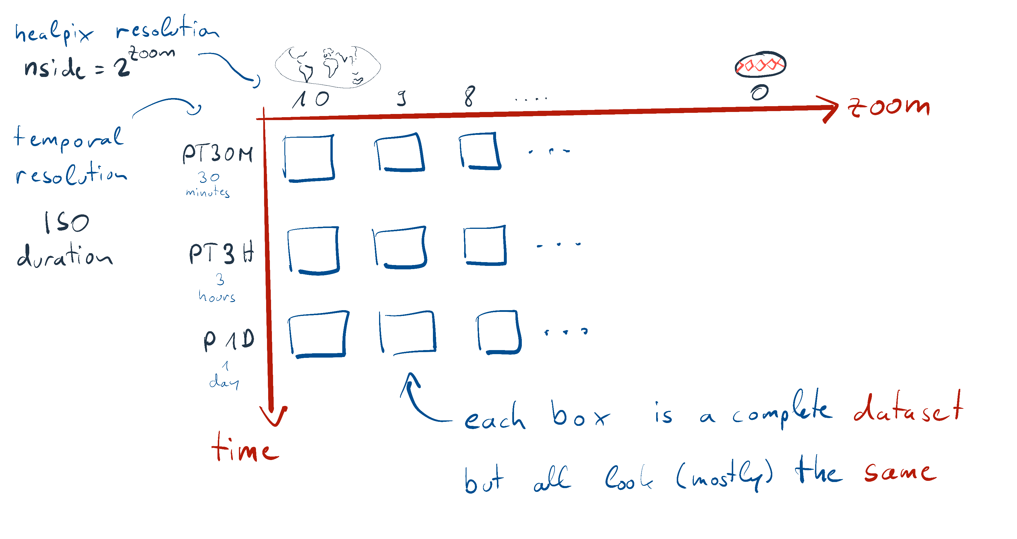
So while technically, there’s an independent Dataset for each combination of the zoom and time parameters, it’s better to picture all the datasets as copies of the same thing, only their coordinates are of course different due to the different resolutions.
The only exception being, that some variables are missing in finer temporal resolutions (e.g. ocean and 3D variables), but generally all variables available at fine resolutions are also available at coarse resolutions.
Let’s see which parameter values are available (you can ommit the pandas part, but it looks nicer):
import pandas as pd

pd.DataFrame(cat.ICON.ngc3028.describe()["user_parameters"])
| name | description | type | allowed | default | |
|---|---|---|---|---|---|
| 0 | time | time resolution of the dataset | str | [PT30M, PT3H, P1D] | P1D |
| 1 | zoom | zoom resolution of the dataset | int | [7, 6, 5, 4, 3, 2, 1, 0] | 0 |
So just as in the picture above, we have time and zoom parameters.
time resolution is given as ISO duration strings, zoom are the number of bisections in the healpix grid (e.g. the data will have \(12 \cdot 4^{zoom}\) cells).
The coarsest settings are the default.
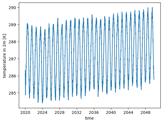
The default is well suited to e.g. obtain the trend of global mean surface temperatures:
ds.tas.mean("cell").plot()
[<matplotlib.lines.Line2D at 0x7fa7c86fc550>]
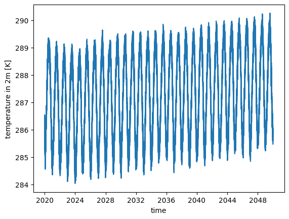
If you are interested in daily variablility, it might however be important to change temporal resolution to a finer scale:
ds_fine = cat.ICON.ngc4008(time="PT3H").to_dask()
ds_fine.tas.mean("cell").plot()
[<matplotlib.lines.Line2D at 0x7fa7c878f250>]
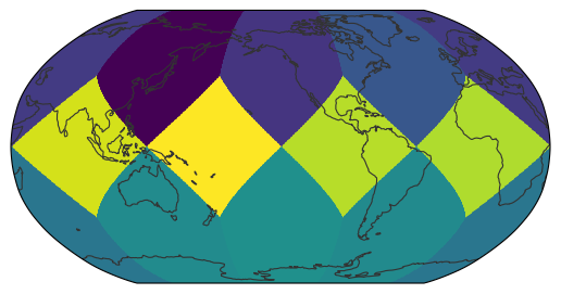
For sure, the 12 horizontal cells won’t provide a detailed map, but let’s check quickly.
We’ll use eaysgems’s plotting tools for their simplicity.
Also we use .isel(time=0) to select the first output timestep by index:
import easygems.healpix as egh


egh.healpix_show(ds.tas.isel(time=0).values)
<matplotlib.image.AxesImage at 0x7fa7c2535940>
For a decent global map, a zoom level of 7 (roughly corresponding to 1x1° resolution) should be good. So let’s try this again:
ds_map = cat.ICON.ngc4008(zoom=7).to_dask()
egh.healpix_show(ds_map.tas.isel(time=0).values)
<matplotlib.image.AxesImage at 0x7fa7c1faf250>
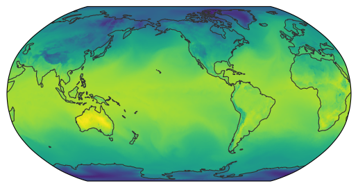
This is a map as we’d expect it to be. You might want to try different zoom settings to get a bit more familiar with the concept. Generally using finer resolutions will load a lot more data, thus it’s recommended to use the coarsest settings suiting your needs.
If your analysis really requires fine resolution data, it might be convenient to use coarse settings while debugging and then switch to finer settings once you are happy with your code.
.to_dask()
While the method for converting a catalog entry into a Dataset is called .to_dask(), it will not return a dask-backed Dataset by default.
In many cases (in particular for doing some quick plots), dask is not really necessary.
As the dask best practices suggest we should Use better algorithms or data structures instead of dask if you don’t need it.
That said, if you need dask (e.g. because of the processing complexity), you can enable it by providing a chunks specification to the catalog.
This can be as simple as cat.ICON.ngc3028(chunks="auto").to_dask().
If you do so, just be sure that your chunk settings are compatible with the underlying storage chunks.
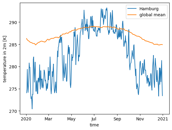
Working with multiple resolutions#
We can also mix resolutions to compare Hamburg’s temperature to the global mean.
To work with multiple resolutions of a single run, it might be useful to store the selected model run’s catalog entry into a variable.
We also need further helper functions to inspect the grid properties provided by the easygems package:
import healpix as hp
import matplotlib.pylab as plt


model_run = cat.ICON.ngc4008

ds_fine = model_run(zoom=7).to_dask()
hamburg = hp.ang2pix(
    egh.get_nside(ds_fine), 9.993333, 53.550556, lonlat=True, nest=egh.get_nest(ds_fine)
)

ds_fine.tas.sel(cell=hamburg, time="2020").plot(label="Hamburg")
model_run(zoom=0).to_dask().tas.sel(time="2020").mean("cell").plot(label="global mean")
plt.legend()
<matplotlib.legend.Legend at 0x7fa7c2537230>
Vertical profile#
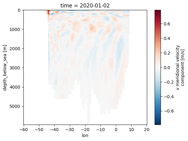
Let’s try something a bit more involved: northward motion of the water across the equator in the atlantic at some point in time:
import numpy as np
import xarray as xr

lons = np.linspace(-60.0, 20.0, 200)
lats = np.full_like(lons, 0.0)

ds = model_run(zoom=7).to_dask()

pnts = xr.DataArray(
    hp.ang2pix(egh.get_nside(ds), lons, lats, lonlat=True, nest=egh.get_nest(ds)),
    dims=("cell",),
    coords={"lon": (("cell",), lons), "lat": (("cell",), lats)},
)

ds.v.isel(time=0, cell=pnts).swap_dims({"cell": "lon"}).plot(x="lon", yincrease=False)
<matplotlib.collections.QuadMesh at 0x7fa7c2537b60>