HEALPix with pyicon#
In this notebook we want to explore how to plot data written out on the HEALPix grid by using pyicon.
In case, you do not know pyicon, it is hosted here: https://gitlab.dkrz.de/m300602/pyicon
Documentation about pyicon can be found here (note the documentation is partly outdated but hopefully will soon be updated): https://m300602.gitlab-pages.dkrz.de/pyicon/
import pyicon as pyic
import matplotlib.pyplot as plt
import numpy as np
import xarray as xr
import cartopy.crs as ccrs
import intake
import cmocean
Load some data via an intake catalog:
# open the intake catalog, decide which model, simulation, outputstream and zoom level to pick
cat = intake.open_catalog(f"https://data.nextgems-h2020.eu/catalog.yaml")
ds = cat["ICON"]["ngc3028"](zoom=7).to_dask()
# ds is an xarray dataset which contains many variables of the particular simulation
ds
<xarray.Dataset>
Dimensions:                              (time: 2010, depth_half: 129,
                                          cell: 196608, level_full: 90, crs: 1,
                                          depth_full: 128,
                                          soil_depth_water_level: 5,
                                          level_half: 91,
                                          soil_depth_energy_level: 5)
Coordinates:
  * crs                                  (crs) float32 nan
  * depth_full                           (depth_full) float32 1.0 ... 5.904e+03
  * depth_half                           (depth_half) float32 0.0 ... 6.003e+03
  * level_full                           (level_full) int32 1 2 3 4 ... 88 89 90
  * level_half                           (level_half) int32 1 2 3 4 ... 89 90 91
  * soil_depth_energy_level              (soil_depth_energy_level) float32 0....
  * soil_depth_water_level               (soil_depth_water_level) float32 0.0...
  * time                                 (time) datetime64[ns] 2020-01-21 ......
    zg                                   (level_full, cell) float32 ...
    zghalf                               (level_half, cell) float32 ...
Dimensions without coordinates: cell
Data variables: (12/92)
    a_tracer_v_to                        (time, depth_half, cell) float32 ...
    atmos_fluxes_frshflux_evaporation    (time, cell) float32 ...
    atmos_fluxes_frshflux_precipitation  (time, cell) float32 ...
    atmos_fluxes_frshflux_runoff         (time, cell) float32 ...
    atmos_fluxes_frshflux_snowfall       (time, cell) float32 ...
    atmos_fluxes_heatflux_latent         (time, cell) float32 ...
    ...                                   ...
    va                                   (time, level_full, cell) float32 ...
    vas                                  (time, cell) float32 ...
    w                                    (time, depth_half, cell) float32 ...
    wa_phy                               (time, level_half, cell) float32 ...
    wind_speed_10m                       (time, cell) float32 ...
zos (time, cell) float32 ...Check dimension and shape of data:
ds.u.dims, ds.u.shape
(('time', 'depth_full', 'cell'), (2010, 128, 196608))
Maps#
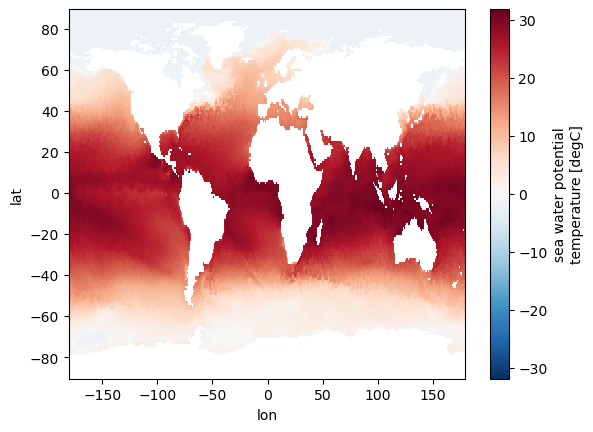
Interpolate to regular grid#
For horizontal maps of data, pyicon interpolates the HEALPix data to a regular grid. This is typically done automatically within the below introduced plotting methods. However, we start here with an example by doing the interpolation explicitly such that it can also be used by other plotting methods.
# interpolation to 1deg regular grid
dai = pyic.hp_to_rectgrid(
    ds.to.isel(time=0, depth_full=0), lon_reg=[-180, 180], lat_reg=[-90, 90], res=1.0
)
dai.dims, dai.shape
(('lat', 'lon'), (180, 360))
# use xarray to plot
dai.plot()
<matplotlib.collections.QuadMesh at 0x7fff89158670>
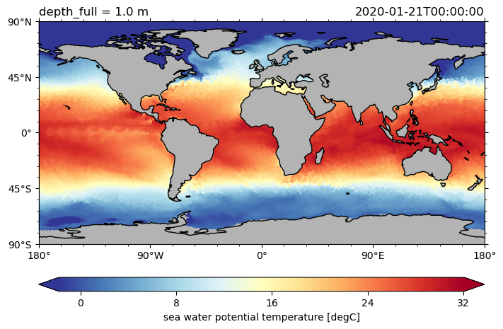
Basic plotting with pyicon#
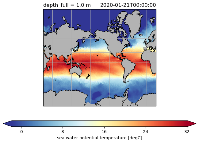
Now, we start using pyicon’s plotting methods. Therefore, we first select a horizontal slice from a variable before plotting it.
da = ds.to.isel(time=0, depth_full=0)
da.pyic.plot()
(<GeoAxes: title={'left': 'depth_full = 1.0 m', 'right': '2020-01-21T00:00:00'}>,
 [<cartopy.mpl.geocollection.GeoQuadMesh at 0x7fff890ef550>,
  <matplotlib.colorbar.Colorbar at 0x7fff8902e170>])
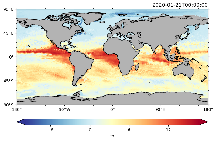
Note that the variable which plotted only needs to be an xarray on the healpix grid. Thus, we can also do mathematical operations and plot the result.
Necessary condition: dimension stays the same, ‘grid_mapping’ attribute is set to ‘crs’ – the latter can probably be omitted in the future.
da = ds.to.isel(time=0).sel(depth_full=0, method="nearest") - ds.to.isel(time=0).sel(
    depth_full=100, method="nearest"
)
da = da.assign_attrs(dict(grid_mapping="crs"))
da.pyic.plot()
(<GeoAxes: title={'right': '2020-01-21T00:00:00'}>,
 [<cartopy.mpl.geocollection.GeoQuadMesh at 0x7fff88df3e50>,
  <matplotlib.colorbar.Colorbar at 0x7fff88cf27a0>])
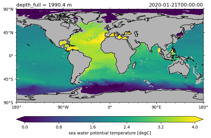
More options and selection methods can also be used
ds.to.isel(time=0).sel(depth_full=2000, method="nearest").pyic.plot(
    cmap="viridis", clim=[0, 4]
)
(<GeoAxes: title={'left': 'depth_full = 1990.4 m', 'right': '2020-01-21T00:00:00'}>,
 [<cartopy.mpl.geocollection.GeoQuadMesh at 0x7fff88a40f70>,
  <matplotlib.colorbar.Colorbar at 0x7fff88b27640>])
Get an overview about what is possible:
pyic.plot?
Signature:
pyic.plot(
    data,
    Plot=None,
    ax=None,
    cax=None,
    asp=None,
    fig_size_fac=2.0,
    mask_data=True,
    logplot=False,
    lon_reg=None,
    lat_reg=None,
    clim='auto',
    cmap='auto',
    conts=None,
    contfs=None,
    clevs=None,
    use_pcol_or_contf=True,
    cincr=-1.0,
    clabel=False,
    xlabel='',
    ylabel='',
    cbar_str='auto',
    cbar_pos='bottom',
    title_right='auto',
    title_left='auto',
    title_center='auto',
    projection='pc',
    coastlines_color='k',
    land_facecolor='0.7',
    axes_facecolor='0.7',
    noland=False,
    gname='auto',
    fpath_tgrid='auto',
    plot_method='nn',
    res=0.3,
    fpath_ckdtree='auto',
    coordinates='clat clon',
    lonlat_for_mask=False,
)
Docstring: <no docstring>
File:      ~/pyicon/pyicon/pyicon_plotting.py
Type:      function
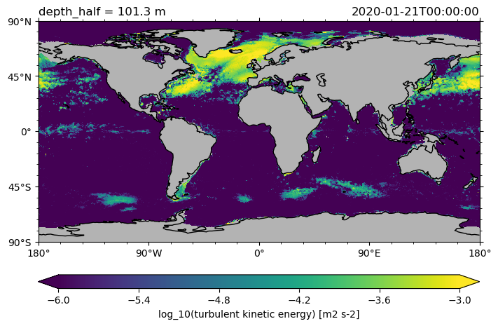
Also the logarithm of a variable can be plotted.
ds.tke.isel(time=0).sel(depth_half=100, method="nearest").pyic.plot(
    cmap="viridis", clim=[-6, -3], logplot=True
)
(<GeoAxes: title={'left': 'depth_half = 101.3 m', 'right': '2020-01-21T00:00:00'}>,
 [<cartopy.mpl.geocollection.GeoQuadMesh at 0x7fff7d8fb100>,
  <matplotlib.colorbar.Colorbar at 0x7fff742ec6a0>])
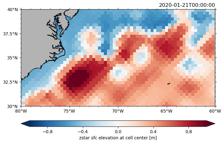
Regional plots#
Select a region by specifying lon_reg, lat_reg.
ds.zos.isel(time=0).pyic.plot(clim=1, lon_reg=[-80, -60], lat_reg=[30, 40])
(<GeoAxes: title={'right': '2020-01-21T00:00:00'}>,
 [<cartopy.mpl.geocollection.GeoQuadMesh at 0x7fff8889d060>,
  <matplotlib.colorbar.Colorbar at 0x7fff888e5780>])
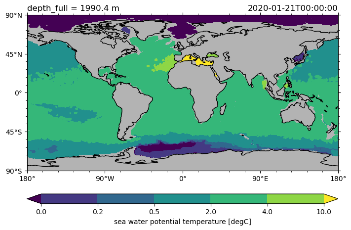
Contour plots#
Per default pcolormesh plots are generated, however also contour or contourf plots can be made.
ds.to.isel(time=0).sel(depth_full=2000, method="nearest").pyic.plot(
    cmap="viridis", contfs=[0, 0.2, 0.5, 2, 4, 10]
)
(<GeoAxes: title={'left': 'depth_full = 1990.4 m', 'right': '2020-01-21T00:00:00'}>,
 [<cartopy.mpl.contour.GeoContourSet at 0x7fff7d39e2f0>,
  <matplotlib.colorbar.Colorbar at 0x7fff7ced58a0>])
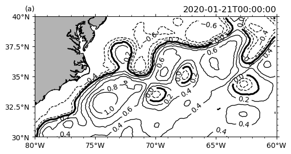
Contour plot
# we need higher resolution for a nice plot
ngc3028 = cat["ICON"]["ngc3028"]
ds_high = ngc3028(zoom=10).to_dask()

P = pyic.Plot(1, 1, plot_cb=False, projection=ccrs.PlateCarree())
ax, cax = P.next()
# use `use_pcol_or_contf=False` to omit any color plot, use `res=0.1` to get high-enourgh resolution to interpolate to
# specify contours by `conts`, use hm[1][0] for contour labels
ax, hm = P.plot(
    ds_high.zos.isel(time=0),
    conts=np.linspace(-1, 1, 11),
    use_pcol_or_contf=False,
    lon_reg=[-80, -60],
    lat_reg=[30, 40],
    res=0.1,
)
P.ax.clabel(hm[0])
P.ax.set_facecolor("w")
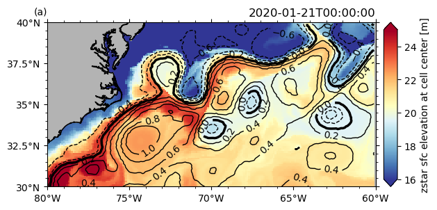
Overlay of a pcolormesh plot and a contour plot.
# make a pcolormesh plot of one variable and a an overlying contour plot with another variable
ngc3028 = cat["ICON"]["ngc3028"]
ds_high = ngc3028(zoom=10).to_dask()

P = pyic.Plot(1, 1, plot_cb=True, projection=ccrs.PlateCarree())
ax, cax = P.next()
P.plot(
    ds_high.to.isel(time=0, depth_full=0),
    clim=[16, 25],
    lon_reg=[-80, -60],
    lat_reg=[30, 40],
    res=0.1,
)
hm = P.plot(
    ds_high.zos.isel(time=0),
    conts=np.linspace(-1, 1, 11),
    use_pcol_or_contf=False,
    lon_reg=[-80, -60],
    lat_reg=[30, 40],
    res=0.1,
)
P.ax.clabel(hm[1][0])
<a list of 28 text.Text objects>
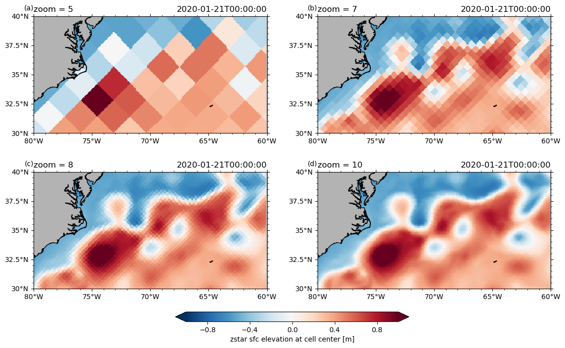
Different zoom levels#
ngc3028 = cat["ICON"]["ngc3028"]
# test different zoom levels
P = pyic.Plot(2, 2, plot_cb="bottom", sharex=False, projection=ccrs.PlateCarree())

for zoom in [5, 7, 8, 10]:
    print(zoom, end="\r")
    ax, cax = P.next()
    # ngc3028(zoom=zoom).to_dask().zos.isel(time=0).pyic.plot(ax=ax, cax=cax, clim=1, lon_reg=[-80,-60], lat_reg=[30,40], cbar_pos='bottom')
    P.plot(
        ngc3028(zoom=zoom).to_dask().zos.isel(time=0),
        clim=1,
        lon_reg=[-80, -60],
        lat_reg=[30, 40],
        res=0.1,
    )
    ax.set_title(f"zoom = {zoom}", loc="left")
10
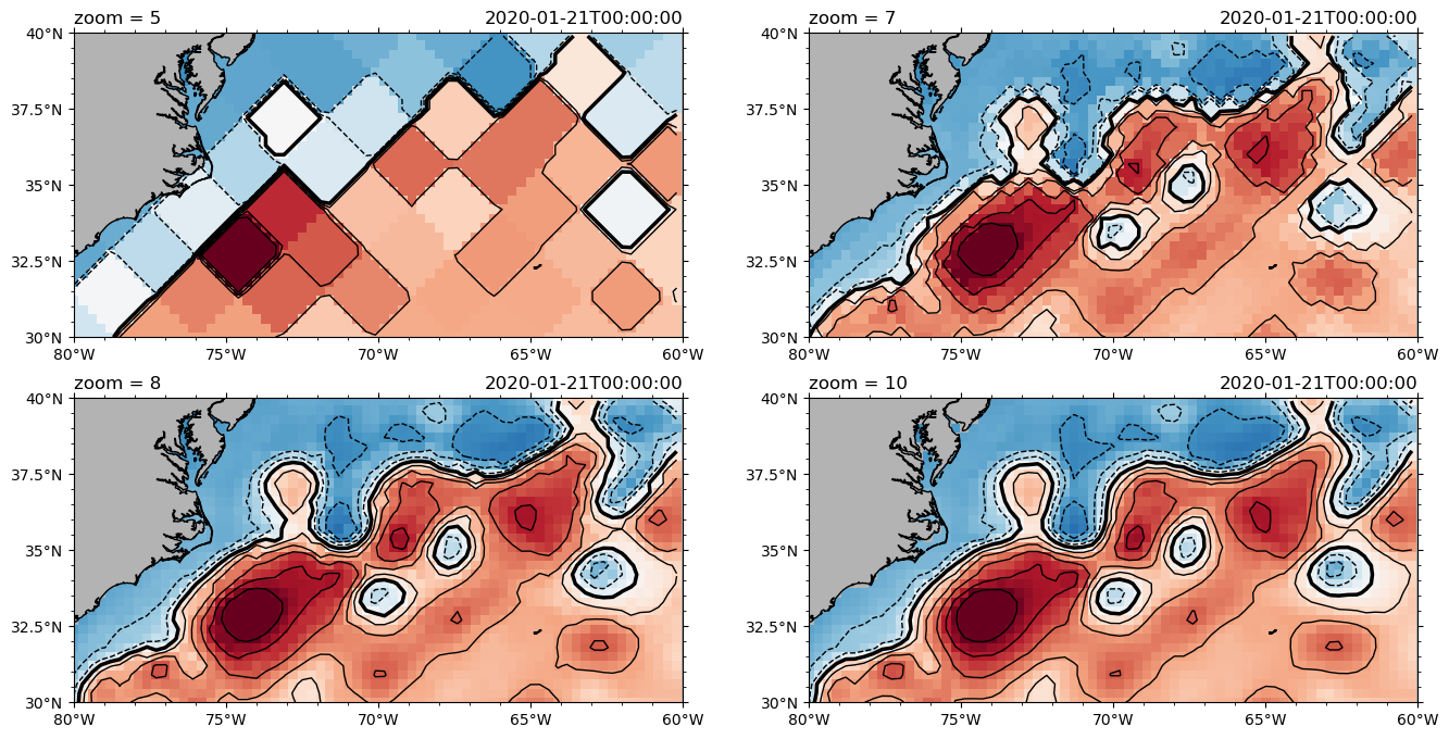
# test different zoom levels with pcolormesh + contours
fig = plt.figure(figsize=(16, 8))

for nn, zoom in enumerate([5, 7, 8, 10]):
    print(zoom, end="\r")
    ax = fig.add_subplot(2, 2, nn + 1, projection=ccrs.PlateCarree())
    ngc3028(zoom=zoom).to_dask().zos.isel(time=0).pyic.plot(
        ax=ax,
        cax=0,
        clim=1,
        lon_reg=[-80, -60],
        lat_reg=[30, 40],
        cbar_pos="bottom",
        conts="auto",
    )
    ax.set_title(f"zoom = {zoom}", loc="left")
10
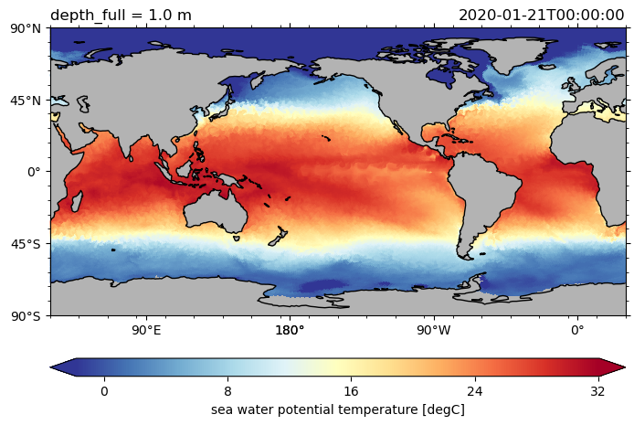
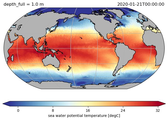
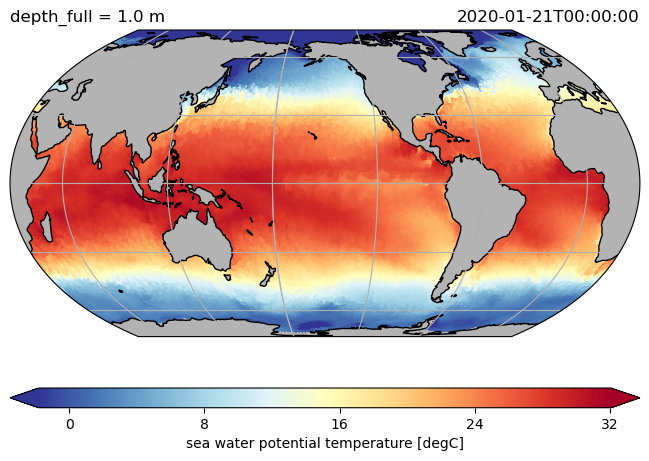
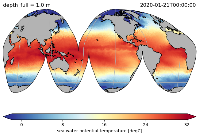
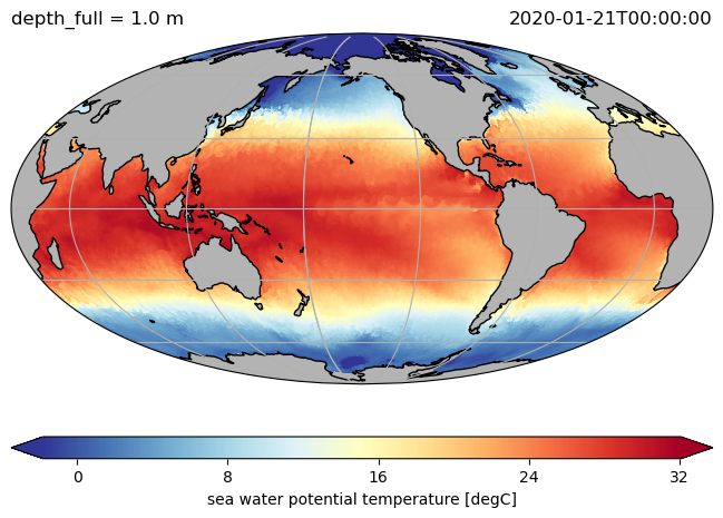
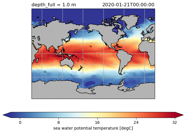
Different projections#
%%time
central_longitude = -150
proj_test = [
    ccrs.PlateCarree(central_longitude=central_longitude),
    ccrs.Robinson(central_longitude=central_longitude),
    ccrs.EqualEarth(central_longitude=central_longitude),
    ccrs.InterruptedGoodeHomolosine(central_longitude=central_longitude),
    ccrs.Mercator(central_longitude=central_longitude),
    ccrs.Mollweide(central_longitude=central_longitude),
    ccrs.Miller(central_longitude=central_longitude),
]

for proj in proj_test:
    # P = pyic.Plot(1, 1, plot_cb=True, projection=proj)
    # P.plot(ds.to.isel(time=0, depth_full=0))
    ds.to.isel(time=0, depth_full=0).pyic.plot(projection=proj)
CPU times: user 1min 26s, sys: 233 ms, total: 1min 26s
Wall time: 1min 27s
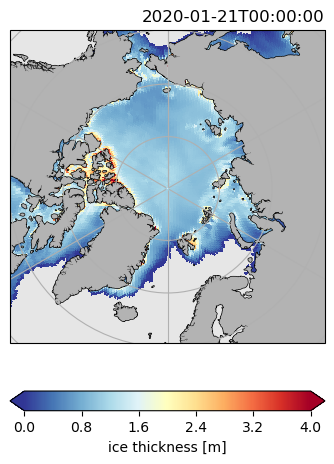
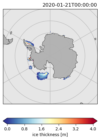
ds.hi.isel(time=0).pyic.plot(clim=[0, 4], projection="np", axes_facecolor="0.9")
(<GeoAxes: title={'right': '2020-01-21T00:00:00'}>,
 [<cartopy.mpl.geocollection.GeoQuadMesh at 0x7fff6fae7460>,
  <matplotlib.colorbar.Colorbar at 0x7fff6faed9f0>])
ds.hi.isel(time=0).pyic.plot(clim=[0, 4], projection="sp", axes_facecolor="0.9")
(<GeoAxes: title={'right': '2020-01-21T00:00:00'}>,
 [<cartopy.mpl.geocollection.GeoQuadMesh at 0x7fff6fbc0910>,
  <matplotlib.colorbar.Colorbar at 0x7fff6f9c1510>])
Sections#
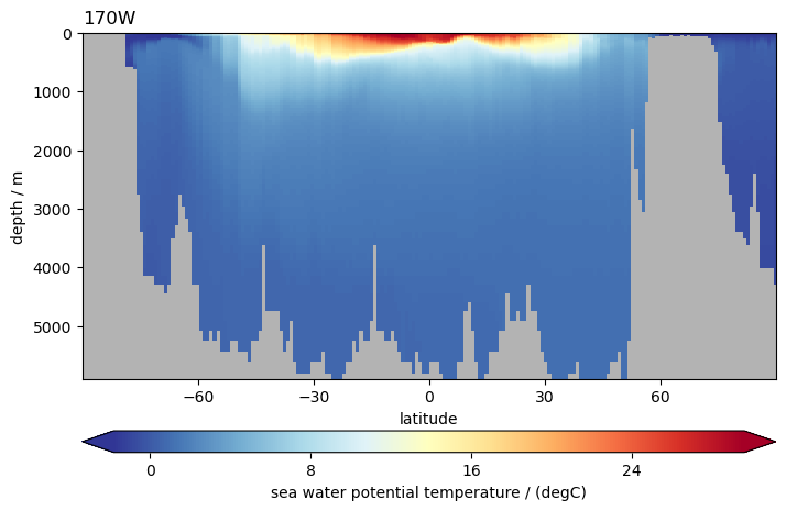
# use plot_sec for plotting section, specify section along const lon by `section` ending with W or E
ds.to.isel(time=0).pyic.plot_sec(section="170W", plot_method="healpix")
(<Axes: title={'left': '170W'}, xlabel='latitude', ylabel='depth / m'>,
 [<matplotlib.collections.QuadMesh at 0x7fff6f734dc0>,
  <matplotlib.colorbar.Colorbar at 0x7fff6f75d450>])
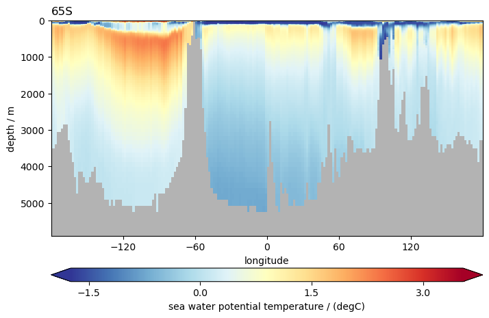
# use plot_sec for plotting section, specify section along const lat by `section` ending with N or S
ds.to.isel(time=0).pyic.plot_sec(section="65S", plot_method="healpix")
(<Axes: title={'left': '65S'}, xlabel='longitude', ylabel='depth / m'>,
 [<matplotlib.collections.QuadMesh at 0x7fff6f610340>,
  <matplotlib.colorbar.Colorbar at 0x7fff6f638670>])
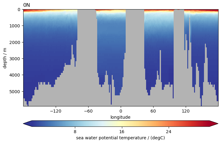
ds.to.isel(time=0).pyic.plot_sec(section="0N", plot_method="healpix")
(<Axes: title={'left': '0N'}, xlabel='longitude', ylabel='depth / m'>,
 [<matplotlib.collections.QuadMesh at 0x7fff6f6a36a0>,
  <matplotlib.colorbar.Colorbar at 0x7fff6f6cbe50>])
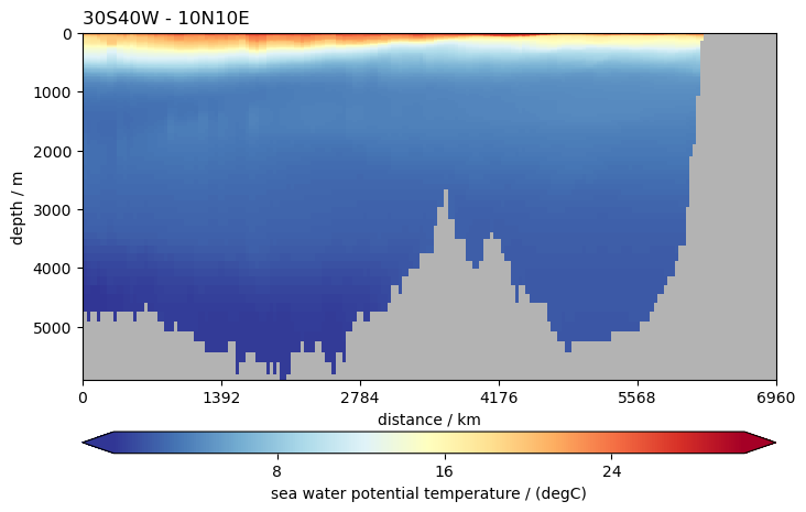
# specify an arbitrary section by specifying `section = 'first_point - last_point'`,
# where first_point has first North/South component and then East/West component
ds.to.isel(time=0).pyic.plot_sec(section="30S40W - 10N10E", plot_method="healpix")
(<Axes: title={'left': '30S40W - 10N10E'}, xlabel='distance / km', ylabel='depth / m'>,
 [<matplotlib.collections.QuadMesh at 0x7fff6f555f30>,
  <matplotlib.colorbar.Colorbar at 0x7fff6f58e5c0>])
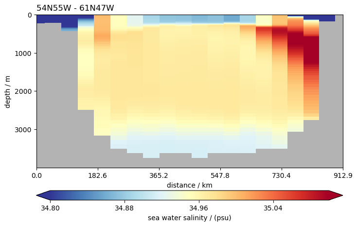
ds.so.isel(time=0).pyic.plot_sec(
    section="54N55W - 61N47W",
    ylim=[0, 4000],
    plot_method="healpix",
    clim=[34.8, 35.1],
    npoints=20,
)
(<Axes: title={'left': '54N55W - 61N47W'}, xlabel='distance / km', ylabel='depth / m'>,
 [<matplotlib.collections.QuadMesh at 0x7fff6f421270>,
  <matplotlib.colorbar.Colorbar at 0x7fff6f451990>])
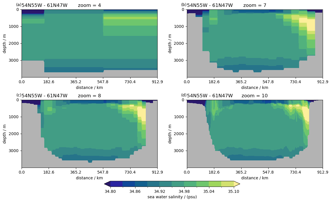
Different zoom levels#
%%time
P = pyic.Plot(2, 2, plot_cb="bottom", sharex=False)

for zoom in [4, 7, 8, 10]:
    print(zoom, end="\r")
    ax, cax = P.next()
    P.plot_sec(
        ngc3028(zoom=zoom).to_dask().so.isel(time=0),
        section="54N55W - 61N47W",
        ylim=[0, 4000],
        plot_method="healpix",
        cmap=cmocean.cm.haline,
        clim=[34.8, 35.1],
    )
    ax.set_title(f"zoom = {zoom}")
CPU times: user 4.34 s, sys: 2.36 s, total: 6.7 s
Wall time: 19.8 s

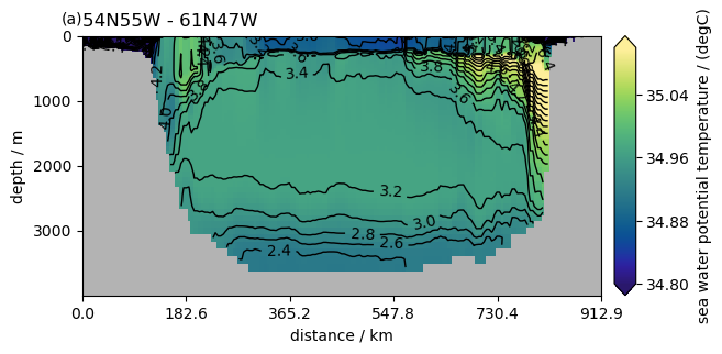
Contour plots#
P = pyic.Plot(1, 1, plot_cb=True)
ax, cax = P.next()

# pcolormesh plot of salinity
ax, hm = P.plot_sec(
    ngc3028(zoom=zoom).to_dask().so.isel(time=0),
    section="54N55W - 61N47W",
    ylim=[0, 4000],
    plot_method="healpix",
    cmap=cmocean.cm.haline,
    clim=[34.8, 35.1],
)
# black contours of temperature
ax, hm = P.plot_sec(
    ngc3028(zoom=zoom).to_dask().to.isel(time=0),
    section="54N55W - 61N47W",
    ylim=[0, 4000],
    plot_method="healpix",
    conts=np.arange(-2, 8, 0.2),
    use_pcol_or_contf=False,
)
P.ax.clabel(hm[0])
<a list of 51 text.Text objects>
%%time
P = pyic.Plot(2, 2, plot_cb="bottom", sharex=False)

for zoom in [4, 7, 8, 10]:
    print(zoom, end="\r")
    ax, cax = P.next()
    P.plot_sec(
        ngc3028(zoom=zoom).to_dask().so.isel(time=0),
        section="54N55W - 61N47W",
        ylim=[0, 4000],
        plot_method="healpix",
        cmap=cmocean.cm.haline,
        clim=[34.8, 35.1],
        contfs="auto",
    )
    ax.set_title(f"zoom = {zoom}")
CPU times: user 3.4 s, sys: 2.27 s, total: 5.67 s
Wall time: 3.63 s
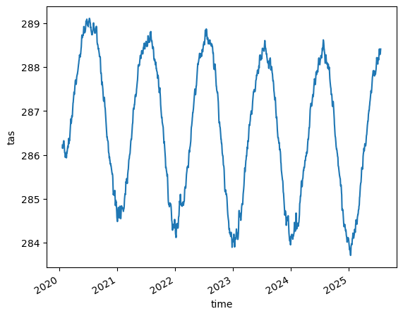
Time series plots#
(no pyicon necessary so far)
ngc3028 = cat["ICON"]["ngc3028"]
%%time
tas = ngc3028(zoom=0).to_dask().tas
tas = tas.compute()
tas.dims, tas.shape
CPU times: user 257 ms, sys: 474 ms, total: 731 ms
Wall time: 51.1 s
(('time', 'cell'), (2010, 12))
tas.mean(dim="cell").plot()
[<matplotlib.lines.Line2D at 0x7fff7d3073d0>]