Using land-sea mask

In this example, it is shown how to use a land-sea mask. We’ll use binary masks on the surface level, which can be extracted from the variable ocean_fraction_surface. Throughout these exercises we will use the land-sea mask to plot

• a spatial map of precipitation over land

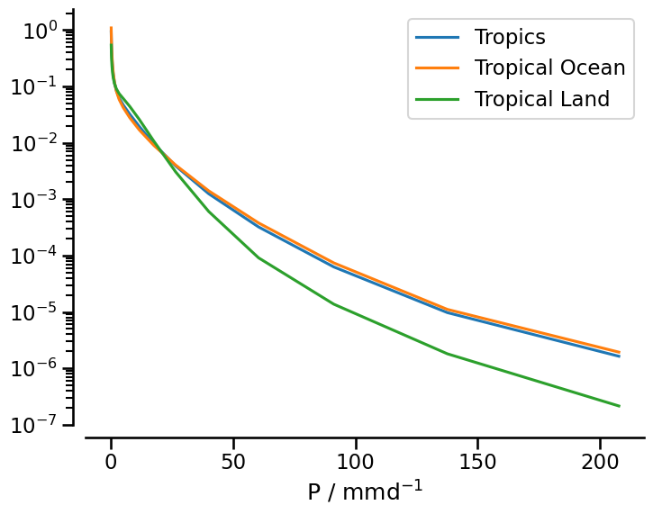
• a probability density function of precipitation over the tropics, tropical land and tropical ocean

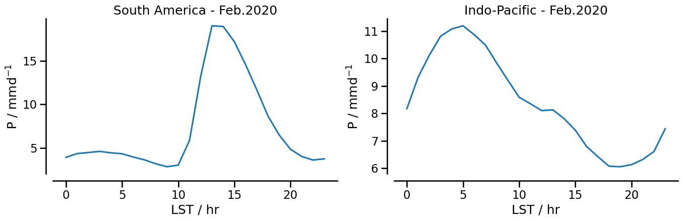
• the diurnal cycle of precipitation over South America and over the Indo-Pacific

Preparations

Importing packages

import intake
import cartopy.crs as ccrs
import cmocean
import healpy as hp
import easygems.healpix as egh
import matplotlib.pyplot as plt
import numpy as np
import seaborn as sns

Getting and selecting data

We pick a nextgems run from the catalog as usual. Furthermore, we keep exp_name and a time_slice of interest for later usage.

cat = intake.open_catalog("https://data.nextgems-h2020.eu/catalog.yaml")
exp_name = "ngc3028"
experiment = cat.ICON[exp_name]
time_slice = slice("2020-02-01", "2020-03-31")

Helper functions

We define some helper functions, which * use the easygems library to attach the locations of the grid cells * change the units of the precipitation variable pr to better fit the upcoming analysis

def preprocess(ds):
    """
    Adapts dataset to the needs of this notebook.
    """
    return ds.pipe(egh.attach_coords).assign(
        pr=(ds.pr * 86400).assign_attrs(units="mm d-1")
    )

masks for specific regions

The purpose of this article is to look at the data based on some regions, so let’s define region masks as functions of a dataset, thus the masks can automatically adapt to the chosen zoom level of the dataset.

def tropics(ds):
    return np.abs(ds.lat) <= 30.1


def land(ds):
    return ds.ocean_fraction_surface == 0


def ocean(ds):
    return ds.ocean_fraction_surface == 1


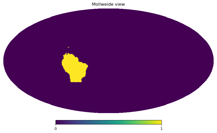
def south_america(ds):
    return tropics(ds) & (ds.lon >= 280) & (ds.lon <= 330) & land(ds)


def indo_pacific(ds):
    return (np.abs(ds.lat) <= 10) & (ds.lon >= 80) & (ds.lon <= 150) & ocean(ds)

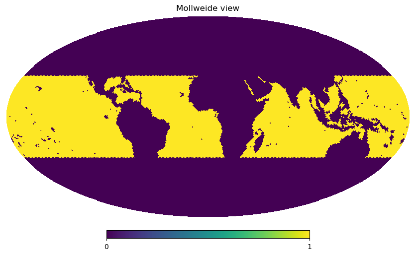
testing the masks

It’s always good to check if those masks we’ve defined actually correspond to the regions we are interested in. For testing, we need a dataset. As the result of the mask function is a boolean mask (i.e. 0 and 1 values) on the healpix grid, we can quickly visualize them using healpy functions:

ds = experiment(zoom=6, chunks="auto").to_dask().pipe(preprocess)
hp.mollview(tropics(ds) & ocean(ds), nest=True, flip="geo")

hp.mollview(south_america(ds), nest=True, flip="geo")

Plotting settings

from cartopy.mpl.ticker import LongitudeFormatter, LatitudeFormatter

proj = ccrs.PlateCarree(central_longitude=-135.5808361)
sns.set_context("talk")  # make plots nicer

Plots

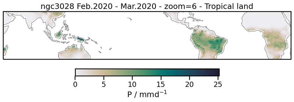
Tropical land precipitation

To get data only for grid cells in the tropics and on land, we can combine the tropics and the land mask using &. We use .pipe(preprocess) to apply our preprocessing function defined above.

%%time
ds = (
    experiment(zoom=6, time="P1D", chunks="auto")
    .to_dask()
    .pipe(preprocess)
    .sel(time=time_slice)
)

pr_tropics_land = ds["pr"].where(tropics(ds) & land(ds)).mean("time")

CPU times: user 145 ms, sys: 3.61 ms, total: 149 ms
Wall time: 152 ms

We can now plot the selected data:

%%time
title = f"{exp_name} Feb.2020 - Mar.2020 - zoom=6 - Tropical land"
fig, ax = plt.subplots(
    figsize=(12, 8), facecolor="white", subplot_kw={"projection": proj}
)
ax.set_extent([-180, 180, -30, 30], crs=ccrs.PlateCarree())
artist = egh.healpix_show(pr_tropics_land, ax=ax, cmap=cmocean.cm.rain)
ax.coastlines(color="gray", lw=1)
fig.colorbar(
    artist, label="P / mmd$^{-1}$", shrink=0.5, orientation="horizontal", pad=0.05
)
plt.title(title)
None

CPU times: user 512 ms, sys: 450 ms, total: 962 ms
Wall time: 15.2 s

PDF of precipitation

Here, we want to look at differences in rain intensity between ocean and land areas within the tropics. To do so, we’ll apply the same masks from above, but look at histograms instead of maps. Let’s get some data first:

ds_hist = (
    experiment(zoom=6, time="P1D")
    .to_dask()
    .pipe(preprocess)
    .sel(time=slice("2020-02-01", "2021-01-31"))
)

Calculating histogram

bins = np.logspace(np.log10(0.1), np.log10(250), 20)
histogram_tropics, _ = np.histogram(
    ds_hist.pr.where(tropics(ds_hist)), bins, density=True
)
histogram_tropics_ocean, _ = np.histogram(
    ds_hist.pr.where(tropics(ds_hist) & ocean(ds_hist)), bins, density=True
)
histogram_tropics_land, _ = np.histogram(
    ds_hist.pr.where(tropics(ds_hist) & land(ds_hist)), bins, density=True
)

xaxis = (bins[1:] + bins[:-1]) / 2
fig, ax = plt.subplots(figsize=(8, 6), facecolor="white")
plt.plot(xaxis, histogram_tropics, label="Tropics")
plt.plot(xaxis, histogram_tropics_ocean, label="Tropical Ocean")
plt.plot(xaxis, histogram_tropics_land, label="Tropical Land")
ax.set_yscale("log")
ax.set_xlabel("P / mmd$^{-1}$")
sns.despine(offset=10)
plt.legend()

<matplotlib.legend.Legend at 0x7fff85a803a0>

Diurnal cycle of precipitation

For this example, we use data with a time step of 30 minutes to calculate the dirunal cycle of precipitation over two regions: South America and the Indo-Pacific. Because data with time step of 30 minutes do not have the variableocean_fraction_surface, we use the daily output to extract this variable and add it to the 30 minutes time step.

%%time
ds_diurnal = (
    experiment(zoom=6, time="PT30M", chunks="auto")
    .to_dask()
    .pipe(preprocess)
    .sel(time=slice("2020-02-01", "2020-02-29"))
)
# unfortunately, ocean_fraction_surface is only available in daily output. Let's fix that:
ds_diurnal = ds_diurnal.assign(
    ocean_fraction_surface=experiment(zoom=6, time="P1D")
    .to_dask()
    .ocean_fraction_surface
)

CPU times: user 106 ms, sys: 13.3 ms, total: 120 ms
Wall time: 246 ms

We’ll group the data by the hour of the day and average over those datapoints over time from every day within our selection:

%%time
pr_samerica_28 = (
    ds_diurnal["pr"].where(south_america(ds_diurnal)).groupby("time.hour").mean()
)

pr_indopacific_28 = (
    ds_diurnal["pr"].where(indo_pacific(ds_diurnal)).groupby("time.hour").mean()
)

CPU times: user 96.3 ms, sys: 5.71 ms, total: 102 ms
Wall time: 104 ms

Calculating diurnal cycle of precipitation

Now, while we have the data grouped by hour, it’s the UTC hour and not the local time of the day. Before averaging horizontally in space, we have to shift every grid cell’s time to local time. We’ll do so by converting the cell’s longitude to a time offset and the modulo operator. We could have done this before the first time-average, but that would create a very large intermediate time variable for each grid cell and all points in time. Doing it in two steps can save a bit of memory.

def local_hour(data):
    return np.round(data.hour + data.lon * (24 / 360)) % 24


def d_cycle(data):
    return data.groupby(local_hour(data)).mean()

%%time
dcycle_samerica_28 = d_cycle(pr_samerica_28)
dcycle_indopacific_28 = d_cycle(pr_indopacific_28)

CPU times: user 1.41 s, sys: 111 ms, total: 1.52 s
Wall time: 1.53 s

def format_axes_time_series(ax, title):
    ax.spines.right.set_visible(False)
    ax.spines.top.set_visible(False)
    ax.set_xlabel("LST / hr")
    ax.set_ylabel("P / mmd$^{-1}$")
    ax.set_title(title)
    sns.despine(offset=10)

fig, (ax1, ax2) = plt.subplots(1, 2, figsize=(16, 4), facecolor="white")
ax1.plot(dcycle_samerica_28)
format_axes_time_series(ax1, title="South America - Feb.2020")

ax2.plot(dcycle_indopacific_28)
format_axes_time_series(ax2, title="Indo-Pacific - Feb.2020")