Averages of ocean data

While we provide atmosphere and ocean data on the same HEALPix grid, handling ocean data requires some special care due to the border between land and ocean. At the finest output grid resolution, we treat a cell either as completely ocean or as completely land, but during coarsening steps, a grid cell can be partially ocean and partially land.

The coarse ocean data contains aggregations of only the ocean (or more generally non-NaN cells), thus e.g. the ocean temperature on a grid cell on the border will still contain the correct ocean temperature. However when doing spatial (e.g. global) averages, partial ocean cells need to be weighted less than fully covered cells to obtain the right result.

import intake

cat = intake.open_catalog("https://data.nextgems-h2020.eu/catalog.yaml")
experiment = cat.ICON.ngc3028

doing it wrong

Let’s first have a look at what would happen if we’d just compute a mean over all the cells for different zoom levels:

import matplotlib.pylab as plt

for zoom in range(11):
    ws = experiment(zoom=zoom).to_dask().wind_speed_10m.sel(time="2020-01")
    ws.mean("cell").plot(label=zoom)
plt.legend()
plt.title("(WRONG) global average over zoom levels")
None

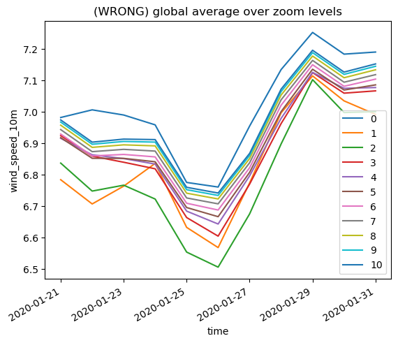
… we get wildly different results, across zoom levels. There is some convergence towards higher resolution because there are proportionally less border cells, but that would of course defeat the purpose of the output hierarchy.

doing it right

So how can we do better?

The dataset provides the area fractions of grid cells covered by ocean in the ocean_fraction_* variables. There’s one variable per vertical grid type. So let’s do a weighted average:

import matplotlib.pylab as plt

for zoom in range(11):
    ds = experiment(zoom=zoom).to_dask()
    ws = ds.wind_speed_10m.sel(time="2020-01")
    ws.weighted(ds.ocean_fraction_surface).mean("cell").plot(label=zoom)
plt.legend()
plt.title("global average over zoom levels")
None

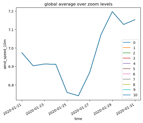
much better! Now we have all globale averages on the same line and thus can use the coarsest zoom level and profit from the output hierarchy.

Be careful with 3D data

There’s a subtle trap for slices of 3D data. If you select a slice out of the data but not out of the weights (and don’t specify the dimension to run the mean along), the code unfortunately works, but gives false results:

import matplotlib.pylab as plt

for zoom in range(11):
    ds = experiment(zoom=zoom).to_dask()
    to = ds.to.isel(time=0, depth_full=0)
    print(to.weighted(ds.ocean_fraction_depth_full).mean().values)

18.749441642680484
18.93881387033061
19.057018612270735
19.089355867021848
19.10544300635326
19.11321655991825
19.11671614014757
19.118259981523554
19.118799459602887
19.118264115458455
19.124199430653736

If you only look at one slice out of the 3D data, you’ll have to subselect the weights as well. Here’s the correct version:

import matplotlib.pylab as plt

for zoom in range(11):
    ds = experiment(zoom=zoom).to_dask()
    to = ds.to.isel(time=0, depth_full=0)
    print(to.weighted(ds.ocean_fraction_depth_full.isel(depth_full=0)).mean().values)

18.578372131136117
18.578370332669174
18.578370332669174
18.578372131136117
18.57836493726835
18.578368534202234
18.578373929603057
18.578370332669174
18.578372131136117
18.57835594493364
18.578350549532814