Torodial Grids on ICON

For idealized simulations ICON uses bi-periodic planar grids. These are often referred to as toroidal grids, or toruses even though their geometry and meta-data is not fully consistent with what one would expect from a torus. For instance they don’t have any curvature.

To understand the torus we plot one such grid created using ICON’s grid generator. It was generated by using the default script for generating a torus, with the parameters 100000 17300 3290 passed to the script. This creates the best fit grid to a domain of 100 km by 17.3 km with an equilateral triangle whose area is the same as a square with side 3290 m. This is the grid that is used to run the aes_bubble configuration of ICON.

Getting the grid

Getting the grid is a bit complicated because we use a premade grid file stored in the DKRZ cloud. A further complication arises because ICON’s grid files adopt the netcdf format, which does not allow them to be opened using http. Hence we need to get using fsspec. If this file were available locally you would not need to use fsspec to first get and cache the file locally, but could replace the grid_url Aby the path to the file locally, and use this directly in the open_dataset call.

import xarray as xr
import fsspec

grid_url = "https://swift.dkrz.de/v1/dkrz_f765c92765f44c068725c0d08cc1e6c5/easyGEMS/icon_bubble_torus.nc"
grid = xr.open_dataset(fsspec.open_local("simplecache::"+grid_url), engine='netcdf4')

Warning!  Library version information error.
The HDF5 library version information are not consistent in its source code.
This is NOT a fatal error but should be corrected.  Setting the environment
variable 'HDF5_DISABLE_VERSION_CHECK' to a value of 1 will suppress
this warning.
Library version information are:
H5_VERS_MAJOR=1, H5_VERS_MINOR=14, H5_VERS_RELEASE=4, H5_VERS_SUBRELEASE=2,
H5_VERS_INFO=HDF5 library version: 1.14.4

Tip

It is pretty straightforward to make your own grid file using the grid-generator. Directions on how to clone the repo, make the generator and create the grid can be found on the repo Wiki. For creating the torus you will want to use grid.create_torus_grid to select the correct runscript template (in the first step under generating grids).

Visualizing the grid structure

import numpy as np
import matplotlib.pyplot as plt

thtmax   = grid.clat_vertices.max()
tht_span = thtmax - grid.clat_vertices.min()
deltht   = grid.clat_vertices[0,2]-grid.clat_vertices[0,0]

vlon = grid.clon_vertices.values[:, [0, 1, 2, 0]]
vlat = grid.clat_vertices.values[:, [0, 1, 2, 0]]
has_lon_wrap = (np.max(vlon, axis=-1) - np.min(vlon, axis=-1)) > np.pi
has_lat_wrap = (np.max(vlat, axis=-1) - np.min(vlat, axis=-1)) > tht_span.values/2
vlon[has_lon_wrap[:, np.newaxis] & (vlon > 0)] -= 2 * np.pi
vlat[has_lat_wrap[:, np.newaxis] & (vlat < 0)] = (thtmax + deltht).values  # TODO: this doesn't match the orginal formula, is that correct?
color = np.where(has_lon_wrap | has_lat_wrap, np.array("dodgerblue"), np.array("k"))

fig, ax = plt.subplots(1,1, sharey=True, figsize = (8,1.75), constrained_layout=True)

for k, (lons, lats, c) in enumerate(zip(vlon, vlat, color)):
    ax.plot(lons,lats,c=c,lw=1.0)
    ax.annotate(f"{k+1}", (np.mean(lons[0:3]), np.mean(lats[0:3])),size=5.,ha='center', va='center',c=c)

About the grid

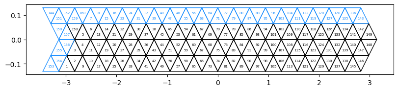
The gird has 160 cells, arranged across 20 columns and 4 rows. A row is comprised of pairs of triangles with opposing polarity, so the total number of cells is \(4\times2\times20=160.\) The \(x\)-axis corresponds to the E-W direction and spans the unit circle from \(-\pi\) to \(\pi\). The \(y\)-axis spans a range of latitudes corresponding to the planar projection of the \(y\) (or North-South) direction on the sphere. Hence the dimensioning of the grid gives it a much smaller angular extent – less than 1/5th of the E-W direction, as height of an equilateral triangle is only \(\sqrt{3}/2\) units width. Hence the grid is \(2\sqrt{3}\) units high and \(20\) units wide.

The toroid can thus be thought of as an equatorial belt, with the caveat that what goes out the north comes in the south.

The blue cells indicate “wrapped” cells, i.e., cells with at least one vertex that enforces periodicity by being connected to the other side of the domain. By definition a point at $\(x=\pi+\varepsilon = -\pi+\varepsilon.\)$ Hence the blue border at the top of the domain connects to the black border on the bottom, and the left quiver-like inset connects to the arrow on the right. Note that every blue triangle touches the vertex of at least one black triangle. This gives the grid its bi-periodicity. The cells are enumerated according to their cell number starting with 1.