The ICON bubble

What is nice about the bubble is that it can be used to test many aspects of the code very quickly. This is because it touches all of the atmospheric physics, it is very quick to run (a 2hr simulation takes 11s on a mac), all the output can be written to make offline debuging easier, it is easy to visualize, and its symmetries help expose errors.

Basic Set-up

The Basic set-up of the bubble consists of an atmosphere over a bi-periodic domain as described here. A roughly 20 km deep atmosphere is discretized over 70 layers and initialized to form two uniformally stratified layers upon which a perturbation is imposed. The first layer extending upwards with a temperature profile given by \(T(z) = T_0 + z\Gamma_0\) to a height \(z_0\) above which the temperature follows the profile \(T(z) = T(z_0) + (z-z_0)\Gamma_1,\) where \(T_0, z_0, \Gamma_0,\) and \(\Gamma_1\) are parameters that can be specified. The humidity is set to a constant prescribed value. The perturbation, or bubble, is specified as a latitudinally slab symmetric gaussian perturbation in relative humidity and temperature that is centered at the surface and the central longitude. The surface is given the propoerties of saturated water at a fixed temperature, and the mean wind is initially set to 0.

The bubble is highly configurable, both in terms of the processes it represents, and in terms of the basic set up. For testing or debugging it is most useful to turn components of ICON on and off, as described below. This helps isolate errors or inconsistencies to particular physical processes, e.g., radiation or turbulent mixing. In terms of the physical set up it is often most useful to vary \(T_0\) (aes_bubble_config%t0 which is set in aes_bubble_nml) and the surface temperature (ape_sst_val which is set in nh_testcase_nml) as this determines the phase of the condensate that forms in the bubble.

An understanding of the bubble is best achieved by reading the code itself. The initialization is performed in src/testcases/mo_aes.bubble.f90, the default parameter settings are set it src/configure_model/mo_aes_bubble.config.f90. The settings can be modified in the namelist, and the grid can be modified by creating a different grid file.

Run the bubble

In the ICON repo, doc/Quick_Start.md provides the 12 commandments of the bubble world (12 commands needed to get the ICON code, configure and make it, configure and then execute the bubble experiment) in the DKRZ environment. The documentation in and referred to by the QuickStart also provides instructions on how to get the bubble running in different environments, or to change the configuration.

Make a nice dataset

The standard bubble ouptut is written to different netcdf files. One of the standard outpouts is 2D model-level output, another has 3D model-level output. Their respective file names are distinguished by the strings atm_2d_ml and atm_3d_ml. Here we combine these data to form single nice data set, with more intuitive coordinates and indexing dimensions.

First some packages are loaded and paths to output are provided. The moist_thermodynamics package is used to specify thermodynamic constants following the prescription used by ICON. Getting the data is complicated by using data on the object store (see here, which we do so the script can be run for everyone. When replicating in your environment the files can be opened using xr.open_dataset(fname) as is customary.

Packages and paths

import numpy as np
import xarray as xr
import matplotlib.pyplot as plt
import seaborn as sns
import pandas as pd

# load thermodynamic variables

from moist_thermodynamics.constants_icon import cpd, rd, cpv, rv, clw, ci, g, lv, ls, Tmelt

cvd = cpd-rd
cvv = cpv-rv
lf  = ls -lv
lvc = lv-(cpv-clw)*Tmelt
lsc = ls-(cpv-ci )*Tmelt

# open 2d and 3d output files created by bubble configuration of ICON

def get_dataset(dataset_name):
    import fsspec
    filename = fsspec.open_local(f"simplecache::https://swift.dkrz.de/v1/dkrz_f765c92765f44c068725c0d08cc1e6c5/easyGEMS/{dataset_name}.nc")
    return xr.open_dataset(filename, engine='netcdf4')

ds2d   = get_dataset("bubble_atm_2d_ml_20080801T000000Z")
ds     = get_dataset("bubble_atm_3d_ml_20080801T000000Z")

Warning!  Library version information error.
The HDF5 library version information are not consistent in its source code.
This is NOT a fatal error but should be corrected.  Setting the environment
variable 'HDF5_DISABLE_VERSION_CHECK' to a value of 1 will suppress
this warning.
Library version information are:
H5_VERS_MAJOR=1, H5_VERS_MINOR=14, H5_VERS_RELEASE=4, H5_VERS_SUBRELEASE=2,
H5_VERS_INFO=HDF5 library version: 1.14.4

Form a single data set

We define a function for calculating the model half levels, which are not part of the standard output. Next we combine the 2D and 3D data, add the half levels, and geometric coordinates. Then dimensions are associated with the new coordinates, and the data set is subsampled to make a single cross section through the latitudes shared by the first cell over the lower atmosphere where the bubble is present.

def add_half_levels(ds):
    nlev = ds.sizes['height']
    zh   = xr.DataArray(np.zeros(nlev+1),dims='height_2',attrs={'long_name' : 'altitude', 'units' : 'km'})
    for k in (np.arange(nlev,0,-1)-1):
        zh[k] = 2*ds.zg[k,0]/1000. - zh[k+1]
    ds['zh'] = zh
    return ds.swap_dims({'height_2' : 'zh'})


for var, da in ds2d.data_vars.items():
    ds[var] = da

ds = add_half_levels(ds)

zg    = (ds.zg[:,0]/1000).assign_attrs({'long_name':'altitude','units':'km'})
xg    = xr.DataArray( ds.clon_bnds[:,1] / np.pi / 2. * 100. + 2.5, dims='ncells', attrs={'long_name' : 'x', 'units' : 'km'})
clat  = xr.DataArray((ds.clat_bnds.mean(dim='vertices').values),dims='ncells')
cond1 = (clat == clat[0].values)

dx = (ds
      .assign_coords({'z' : zg})
      .assign_coords({'x' : xg})
      .where(cond1, drop=True)
      .swap_dims({'height' : 'z'})
      .swap_dims({'ncells' : 'x'})
      .sel(z=slice(6000., 0))
    )

The bubble cross section

Because negligible numerical changes from different implementations will not change the visual appearance of the bubble evolution, it makes the visulalization of the bubble evolution a more intuitive regression test.

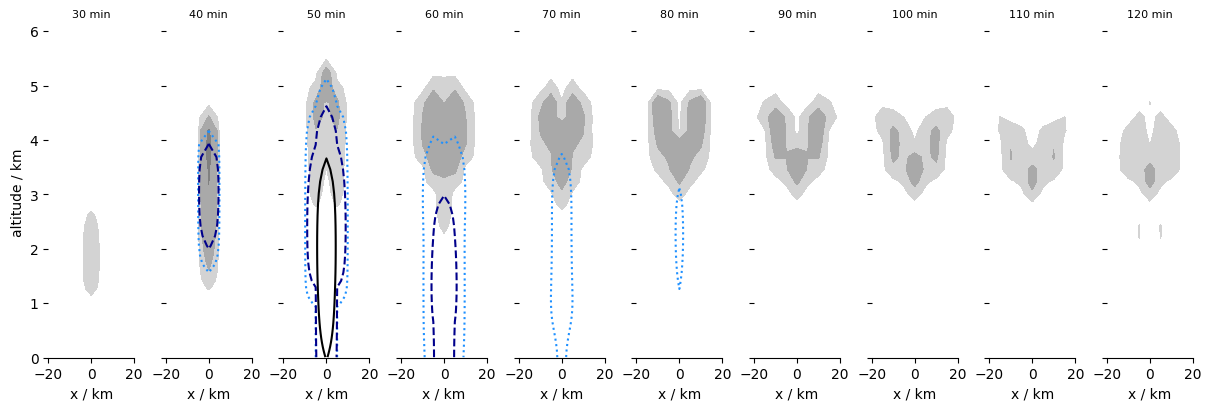
In this example the slice (selected above) across the slab-symmetric dimension of the bubble is plotted at evenly spaced time intervals. To select the times to visualize, we here specify the sampling frequency to be 10 min intervals starting 30 min into the evolution.

time_values = pd.date_range(start="2008-08-01 00:30:00", end="2008-08-01 02:00:00", freq="10min")

Two forms of visualization are considered. The first is designed to emphasize the condensate for the saturated bubble:

fig, axs    = plt.subplots(1, len(time_values) , sharey=True, figsize = (12,4), constrained_layout=True)
for time, ax in zip(time_values, axs):    
    time_elapsed = (dx.time.sel(time=time) - dx.time[0])/np.timedelta64(1,'s') / 60.
    (dx.clw*1000).sel(time=time).plot.contourf(
        ax=ax,
        levels=[0.01,0.2,1.0,4.0,20.],
        colors=['white','lightgrey','darkgrey','grey','black','purple'],
        add_colorbar=False
        )
    (dx.qr*1000).sel(time=time).plot.contour(
        ax=ax,
        levels=[0.01,0.1,1.5],
        colors=['dodgerblue','darkblue','black'],
        linestyles=['dotted','dashed','solid'],
        linewidths=1.5
        )

    sns.despine(offset=0,left=True)
    ax.label_outer()
    ax.set_xlim(-20.,20.)
    ax.set_ylim(  0,6.1)
    ax.set_xlabel(f'{dx.x.long_name} / {dx.x.units}') 
    ax.set_title(f'{time_elapsed:.0f} min',fontsize=8)
    
axs[0].set_ylabel(f'{dx.z.long_name} / {dx.x.units}');

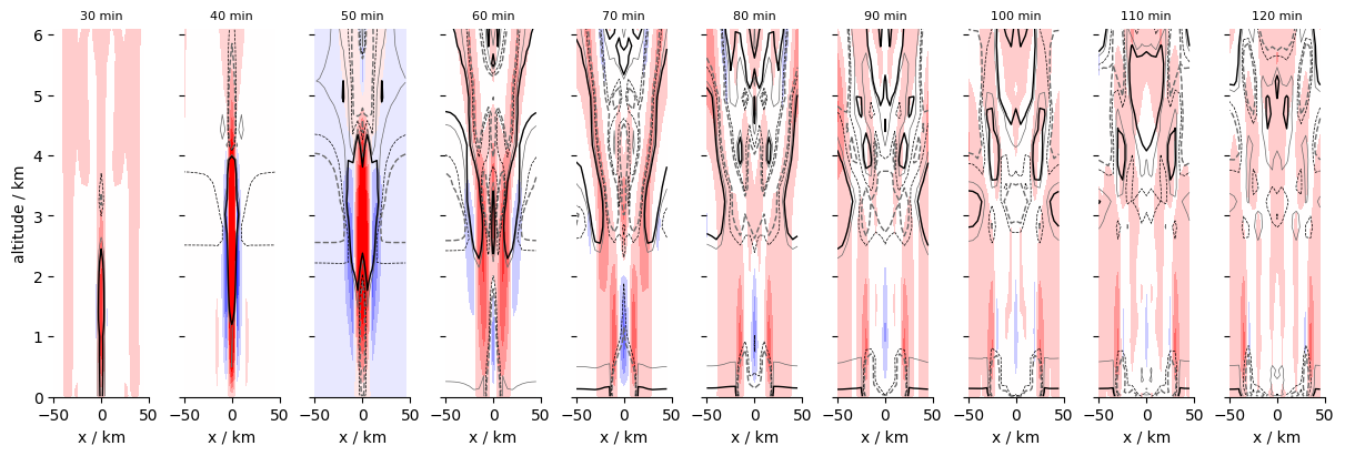
The second emphasize temperature/buoyancy perturbations and the vertical velocity, whereby the latter locates on the half levels.

fig, axs    = plt.subplots(1, len(time_values) , sharey=True, figsize = (12,4), constrained_layout=True)

for time, ax in zip(time_values, axs):    

    time_elapsed = (dx.time.sel(time=time) - dx.time[0])/np.timedelta64(1,'s') / 60.

    w  = dx.wa.sel(time=time)
    qc = (dx.clw + dx.cli + dx.qr + dx.qs + dx.qg).sel(time=time)
    Tv = (dx.ta * (1 + 0.608 * dx.hus - qc)).sel(time=time)
    Tp = (Tv -  Tv.mean(dim='x')) 
    w.plot.contourf(ax=ax, cmap='bwr', levels=np.arange(-3,3,0.5),add_colorbar=False)
    Tp.plot.contour(
        ax         = ax,
        levels     = [-1.0,-0.5,0.5,1.0],
        colors     = ['dimgrey','k'],
        linewidths = [1.0,0.5,0.5,1.0],
        linestyles = ['dashed','dashed','solid','solid']
    )

    sns.despine(offset=0,left=True)
    ax.label_outer()
    ax.set_xlim(-50.,50.)
    ax.set_ylim(  0,6.1)
    ax.set_xlabel(f'{dx.x.long_name} / {dx.x.units}') 
    ax.set_title(f'{time_elapsed:.0f} min',fontsize=8)
    
axs[0].set_ylabel(f'{dx.zh.long_name} / {dx.zh.units}');

Tracking mass

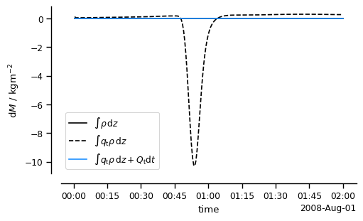
A time-series analysis of domain integrated values also provides a nice check on the code. This example shows how the water mass in the domain changes due to precipitation and evaporation, but that when accounting for the net flux across the lower boundary, mass conservation is maintained.

dz = xr.DataArray(-1000*ds.zh.diff(dim='zh').values,dims='height')
M  = (ds.rho * dz)
Mv = ds.hus * M
Mc = ds.clw * M
Mx = (ds.cli + ds.qr + ds.qg + ds.qs)*M
Mt = Mv + Mc + Mx
Md = M - Mt

dM   = M.diff(dim='time').sum(axis=(1,2))
dMt  = Mt.diff(dim='time').sum(axis=(1,2))
Msfc = (ds.evspsbl+ds.prlr).sum(dim='ncells')*30.
    
sns.set_context('paper')
fig, ax = plt.subplots(1,1, sharey=True, figsize = (5,3),constrained_layout=True)

dM.plot(label='$\\int \\rho \\, \\mathrm{d}z$',c='k')
dMt.plot(label='$\\int q_\\mathrm{t} \\rho \\, \\mathrm{d}z$',c='k',ls='dashed')
(dMt+Msfc).plot(label='$\\int q_\\mathrm{t} \\rho \\, \\mathrm{d}z + Q_\\mathrm{t} \\mathrm{d}t$',c='dodgerblue')

ax.set_ylabel('d$M$ / kgm$^{-2}$') 
plt.legend(ncol=1)
sns.despine(offset=10)

Modifying the bubble

To modify the bubble there are two options.

1. Rename the bubble.config file in the ICON run directory and create a new experiment using mkexp.

2. Modify the runscript directly.

A useful example is the bubble with all of the physics turned off, which following option 1 can be done as follows.

    [[[aes_phy_nml]]]
-      aes_phy_config(1)%dt_mig = $ATMO_TIME_STEP
+      aes_phy_config(1)%dt_rad =" " 
+      aes_phy_config(1)%dt_vdf = " " 
+      aes_phy_config(1)%dt_mig = " " 
...
   [[[output_nml atm_2d]]]
-      ml_varlist = ps, psl, ts, clt, prw, cllvi, clivi, qrvi, qsvi, qgvi, hfls, hfss, evspsbl, prlr, prls, cptgzvi, pr_rain, pr_snow, pr_grpl, pr_ice
+      ml_varlist = ps, psl, ts, clt, prw, cllvi, clivi, qrvi, qsvi, qgvi, hfls, hfss, evspsbl, prlr, prls, cptgzvi

This sets a void time-step for the physical processes, which means that they are no longer called. It also removes variables that no longer exist, i.e., were associated with the evocation of the microphysics.

Tracking energy

In the absence of boundary fluxes total energy, the sum of internal, potential and kinetic energy, should be conserved. This example shows the time evolution of the total energy for the dry bubble configured above.

ds     = get_dataset("dry_bubble_atm_3d_ml_20080801T000000Z")
ds2d   = get_dataset("dry_bubble_atm_2d_ml_20080801T000000Z")

ds = add_half_levels(ds).assign_coords(zg=ds.zg) 
dt = (ds.time.diff(dim='time')/np.timedelta64(1, 's'))

M  = (ds.rho * xr.DataArray(-ds.zh.diff(dim='zh').values,dims='height'))*1000.  # recall zh in km, indexed from top
PE = (ds.zg[:,0] * g * M).sum(dim='height').mean(dim='ncells')
KE = (0.5 * (ds.ua**2 + ds.va**2 + ds.wa.interp(zh=zg)**2) * M).sum(dim='height').mean(dim='ncells')

Tk   = ds.ta
qv   = ds.hus
qliq = ds.clw + ds.qr
qice = ds.cli + ds.qs + ds.qg
qtot = qliq + qice + qv
cx   = cvd*(1-qtot) + cvv*qv + clw*qliq + ci*qice
IE   = ((cx*Tk - qliq*(lv - (cpv-clw)*Tmelt) - qice *(ls- (cpv-ci)*Tmelt)) * M).mean(dim='ncells').sum(dim='height')

dPEdt = PE.diff(dim='time')/dt
dKEdt = KE.diff(dim='time')/dt
dIEdt = IE.diff(dim='time')/dt
dTEdt = dPEdt + dKEdt + dIEdt

sns.set_context('paper')
fig, ax = plt.subplots(1,1, sharey=True, figsize = (5,3),constrained_layout=True)

dIEdt.plot(label='$\\mathrm{d}E_\\mathrm{I}/\\mathrm{d}t$',c='crimson',ls='dotted')
dPEdt.plot(label='$\\mathrm{d}E_\\mathrm{P}/\\mathrm{d}t$',c='dodgerblue',ls='dotted')
dKEdt.plot(label='$\\mathrm{d}E_\\mathrm{K}/\\mathrm{d}t$',c='green',ls='dotted')
dTEdt.plot(label='$\\mathrm{d}E/\\mathrm{d}t$',c='k')

ax.set_ylabel('Power density / Wm$^{-2}$') 
plt.legend(ncol=2)
sns.despine(offset=10)

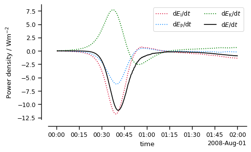
The total energy (solid black line) should not vary over the course of the run. This shows it does. While the model dynamics is good at converting between potential and kinetic energy, it seems that dynamic reductions in kinetic energy that are not balanced by an incrase in potential energy are also not dissipated into internal energy. Variations are on the order of a few W/m2.