Selecting geospatial features#
For scientific analysis it is often required to sample specific parts of the globe, whether geospatial sections or scientific regions of interest.
The HEALPix grid provides an analytical mapping between coordinates and indices, enabling fast and straightforward sampling.
This notebook showcases some of the convenience functions provided by the easygems package.
For demonstration, we will use a remapped version of the ERA5 reanalysis dataset.
import intake
import easygems.healpix as egh


cat = intake.open_catalog("https://data.nextgems-h2020.eu/online.yaml")
ds = cat.ERA5(zoom=6).to_dask()
ds
<xarray.Dataset> Size: 136GB
Dimensions:  (time: 1008, cell: 49152, level: 37)
Coordinates:
  * time     (time) datetime64[ns] 8kB 1940-01-01 1940-02-01 ... 2023-12-01
  * cell     (cell) float32 197kB 0.0 1.0 2.0 ... 4.915e+04 4.915e+04 4.915e+04
  * level    (level) float32 148B 1.0 2.0 3.0 5.0 ... 925.0 950.0 975.0 1e+03
    crs      float32 4B ...
    lat      (cell) float32 197kB dask.array<chunksize=(49152,), meta=np.ndarray>
    lon      (cell) float32 197kB dask.array<chunksize=(49152,), meta=np.ndarray>
Data variables: (12/111)
    100u     (time, cell) float32 198MB dask.array<chunksize=(24, 16384), meta=np.ndarray>
    100v     (time, cell) float32 198MB dask.array<chunksize=(24, 16384), meta=np.ndarray>
    10fg     (time, cell) float32 198MB dask.array<chunksize=(24, 16384), meta=np.ndarray>
    10si     (time, cell) float32 198MB dask.array<chunksize=(24, 16384), meta=np.ndarray>
    10u      (time, cell) float32 198MB dask.array<chunksize=(24, 16384), meta=np.ndarray>
    10v      (time, cell) float32 198MB dask.array<chunksize=(24, 16384), meta=np.ndarray>
    ...       ...
    uvb      (time, cell) float32 198MB dask.array<chunksize=(24, 16384), meta=np.ndarray>
    v        (time, level, cell) float32 7GB dask.array<chunksize=(24, 4, 4096), meta=np.ndarray>
    vo       (time, level, cell) float32 7GB dask.array<chunksize=(24, 4, 4096), meta=np.ndarray>
    w        (time, level, cell) float32 7GB dask.array<chunksize=(24, 4, 4096), meta=np.ndarray>
    z        (time, level, cell) float32 7GB dask.array<chunksize=(24, 4, 4096), meta=np.ndarray>
    zust     (time, cell) float32 198MB dask.array<chunksize=(24, 16384), meta=np.ndarray>
Attributes:
    acknowledgment:  Contains modified Copernicus Climate Change Service info...
    contact:         lukas.kluft@mpimet.mpg.de
    creator:         Lukas Kluft
    description:     HEALPixelation of ERA5
source: Post-processed dataset based on the ERA5 mirror located ...- time: 1008
- cell: 49152
- level: 37
- time(time)datetime64[ns]1940-01-01 ... 2023-12-01
- axis :
- T
array(['1940-01-01T00:00:00.000000000', '1940-02-01T00:00:00.000000000', '1940-03-01T00:00:00.000000000', ..., '2023-10-01T00:00:00.000000000', '2023-11-01T00:00:00.000000000', '2023-12-01T00:00:00.000000000'], shape=(1008,), dtype='datetime64[ns]') - cell(cell)float320.0 1.0 2.0 ... 4.915e+04 4.915e+04
array([0.0000e+00, 1.0000e+00, 2.0000e+00, ..., 4.9149e+04, 4.9150e+04, 4.9151e+04], shape=(49152,), dtype=float32) - level(level)float321.0 2.0 3.0 ... 950.0 975.0 1e+03
- axis :
- Z
- long_name :
- Air pressure at model level
- positive :
- down
- standard_name :
- air_pressure
- units :
- hPa
array([ 1., 2., 3., 5., 7., 10., 20., 30., 50., 70., 100., 125., 150., 175., 200., 225., 250., 300., 350., 400., 450., 500., 550., 600., 650., 700., 750., 775., 800., 825., 850., 875., 900., 925., 950., 975., 1000.], dtype=float32) - crs()float32...
- grid_mapping_name :
- healpix
- healpix_nside :
- 64
- healpix_order :
- nested
[1 values with dtype=float32]
- lat(cell)float32dask.array<chunksize=(49152,), meta=np.ndarray>
- long_name :
- latitude
- standard_name :
- latitude
- units :
- degrees_north
Array Chunk Bytes 192.00 kiB 192.00 kiB Shape (49152,) (49152,) Dask graph 1 chunks in 2 graph layers Data type float32 numpy.ndarray - lon(cell)float32dask.array<chunksize=(49152,), meta=np.ndarray>
- long_name :
- longitude
- standard_name :
- longitude
- units :
- degrees_east
Array Chunk Bytes 192.00 kiB 192.00 kiB Shape (49152,) (49152,) Dask graph 1 chunks in 2 graph layers Data type float32 numpy.ndarray
- 100u(time, cell)float32dask.array<chunksize=(24, 16384), meta=np.ndarray>
- grid_mapping :
- crs
- levtype :
- surface
- long_name :
- 100 metre U wind component
- standard_name :
- units :
- m s**-1
Array Chunk Bytes 189.00 MiB 1.50 MiB Shape (1008, 49152) (24, 16384) Dask graph 126 chunks in 2 graph layers Data type float32 numpy.ndarray - 100v(time, cell)float32dask.array<chunksize=(24, 16384), meta=np.ndarray>
- grid_mapping :
- crs
- levtype :
- surface
- long_name :
- 100 metre V wind component
- standard_name :
- units :
- m s**-1
Array Chunk Bytes 189.00 MiB 1.50 MiB Shape (1008, 49152) (24, 16384) Dask graph 126 chunks in 2 graph layers Data type float32 numpy.ndarray - 10fg(time, cell)float32dask.array<chunksize=(24, 16384), meta=np.ndarray>
- grid_mapping :
- crs
- levtype :
- surface
- long_name :
- 10 metre wind gust since previous post-processing
- standard_name :
- units :
- m s**-1
Array Chunk Bytes 189.00 MiB 1.50 MiB Shape (1008, 49152) (24, 16384) Dask graph 126 chunks in 2 graph layers Data type float32 numpy.ndarray - 10si(time, cell)float32dask.array<chunksize=(24, 16384), meta=np.ndarray>
- grid_mapping :
- crs
- levtype :
- surface
- long_name :
- 10 metre wind speed
- standard_name :
- units :
- m s**-1
Array Chunk Bytes 189.00 MiB 1.50 MiB Shape (1008, 49152) (24, 16384) Dask graph 126 chunks in 2 graph layers Data type float32 numpy.ndarray - 10u(time, cell)float32dask.array<chunksize=(24, 16384), meta=np.ndarray>
- grid_mapping :
- crs
- levtype :
- surface
- long_name :
- 10 metre U wind component
- standard_name :
- units :
- m s**-1
Array Chunk Bytes 189.00 MiB 1.50 MiB Shape (1008, 49152) (24, 16384) Dask graph 126 chunks in 2 graph layers Data type float32 numpy.ndarray - 10v(time, cell)float32dask.array<chunksize=(24, 16384), meta=np.ndarray>
- grid_mapping :
- crs
- levtype :
- surface
- long_name :
- 10 metre V wind component
- standard_name :
- units :
- m s**-1
Array Chunk Bytes 189.00 MiB 1.50 MiB Shape (1008, 49152) (24, 16384) Dask graph 126 chunks in 2 graph layers Data type float32 numpy.ndarray - 2d(time, cell)float32dask.array<chunksize=(24, 16384), meta=np.ndarray>
- grid_mapping :
- crs
- levtype :
- surface
- long_name :
- 2 metre dewpoint temperature
- standard_name :
- units :
- K
Array Chunk Bytes 189.00 MiB 1.50 MiB Shape (1008, 49152) (24, 16384) Dask graph 126 chunks in 2 graph layers Data type float32 numpy.ndarray - 2t(time, cell)float32dask.array<chunksize=(24, 16384), meta=np.ndarray>
- grid_mapping :
- crs
- levtype :
- surface
- long_name :
- 2 metre temperature
- standard_name :
- units :
- K
Array Chunk Bytes 189.00 MiB 1.50 MiB Shape (1008, 49152) (24, 16384) Dask graph 126 chunks in 2 graph layers Data type float32 numpy.ndarray - asn(time, cell)float32dask.array<chunksize=(24, 16384), meta=np.ndarray>
- grid_mapping :
- crs
- levtype :
- surface
- long_name :
- Snow albedo
- standard_name :
- units :
- (0 - 1)
Array Chunk Bytes 189.00 MiB 1.50 MiB Shape (1008, 49152) (24, 16384) Dask graph 126 chunks in 2 graph layers Data type float32 numpy.ndarray - bld(time, cell)float32dask.array<chunksize=(24, 16384), meta=np.ndarray>
- grid_mapping :
- crs
- levtype :
- surface
- long_name :
- Boundary layer dissipation
- standard_name :
- kinetic_energy_dissipation_in_atmosphere_boundary_layer
- units :
- J m**-2
Array Chunk Bytes 189.00 MiB 1.50 MiB Shape (1008, 49152) (24, 16384) Dask graph 126 chunks in 2 graph layers Data type float32 numpy.ndarray - blh(time, cell)float32dask.array<chunksize=(24, 16384), meta=np.ndarray>
- grid_mapping :
- crs
- levtype :
- surface
- long_name :
- Boundary layer height
- standard_name :
- units :
- m
Array Chunk Bytes 189.00 MiB 1.50 MiB Shape (1008, 49152) (24, 16384) Dask graph 126 chunks in 2 graph layers Data type float32 numpy.ndarray - cape(time, cell)float32dask.array<chunksize=(24, 16384), meta=np.ndarray>
- grid_mapping :
- crs
- levtype :
- surface
- long_name :
- Convective available potential energy
- standard_name :
- units :
- J kg**-1
Array Chunk Bytes 189.00 MiB 1.50 MiB Shape (1008, 49152) (24, 16384) Dask graph 126 chunks in 2 graph layers Data type float32 numpy.ndarray - cbh(time, cell)float32dask.array<chunksize=(24, 16384), meta=np.ndarray>
- grid_mapping :
- crs
- levtype :
- surface
- long_name :
- Cloud base height
- standard_name :
- units :
- m
Array Chunk Bytes 189.00 MiB 1.50 MiB Shape (1008, 49152) (24, 16384) Dask graph 126 chunks in 2 graph layers Data type float32 numpy.ndarray - cc(time, level, cell)float32dask.array<chunksize=(24, 4, 4096), meta=np.ndarray>
- grid_mapping :
- crs
- levtype :
- isobaricInhPa
- long_name :
- Fraction of cloud cover
- standard_name :
- units :
- (0 - 1)
Array Chunk Bytes 6.83 GiB 1.50 MiB Shape (1008, 37, 49152) (24, 4, 4096) Dask graph 5040 chunks in 2 graph layers Data type float32 numpy.ndarray - cdir(time, cell)float32dask.array<chunksize=(24, 16384), meta=np.ndarray>
- grid_mapping :
- crs
- levtype :
- surface
- long_name :
- Clear-sky direct solar radiation at surface
- standard_name :
- units :
- J m**-2
Array Chunk Bytes 189.00 MiB 1.50 MiB Shape (1008, 49152) (24, 16384) Dask graph 126 chunks in 2 graph layers Data type float32 numpy.ndarray - ci(time, cell)float32dask.array<chunksize=(24, 16384), meta=np.ndarray>
- grid_mapping :
- crs
- levtype :
- surface
- long_name :
- Sea ice area fraction
- standard_name :
- sea_ice_area_fraction
- units :
- (0 - 1)
Array Chunk Bytes 189.00 MiB 1.50 MiB Shape (1008, 49152) (24, 16384) Dask graph 126 chunks in 2 graph layers Data type float32 numpy.ndarray - ciwc(time, level, cell)float32dask.array<chunksize=(24, 4, 4096), meta=np.ndarray>
- grid_mapping :
- crs
- levtype :
- isobaricInhPa
- long_name :
- Specific cloud ice water content
- standard_name :
- units :
- kg kg**-1
Array Chunk Bytes 6.83 GiB 1.50 MiB Shape (1008, 37, 49152) (24, 4, 4096) Dask graph 5040 chunks in 2 graph layers Data type float32 numpy.ndarray - clwc(time, level, cell)float32dask.array<chunksize=(24, 4, 4096), meta=np.ndarray>
- grid_mapping :
- crs
- levtype :
- isobaricInhPa
- long_name :
- Specific cloud liquid water content
- standard_name :
- units :
- kg kg**-1
Array Chunk Bytes 6.83 GiB 1.50 MiB Shape (1008, 37, 49152) (24, 4, 4096) Dask graph 5040 chunks in 2 graph layers Data type float32 numpy.ndarray - cp(time, cell)float32dask.array<chunksize=(24, 16384), meta=np.ndarray>
- grid_mapping :
- crs
- levtype :
- surface
- long_name :
- Convective precipitation
- standard_name :
- lwe_thickness_of_convective_precipitation_amount
- units :
- m
Array Chunk Bytes 189.00 MiB 1.50 MiB Shape (1008, 49152) (24, 16384) Dask graph 126 chunks in 2 graph layers Data type float32 numpy.ndarray - crr(time, cell)float32dask.array<chunksize=(24, 16384), meta=np.ndarray>
- grid_mapping :
- crs
- levtype :
- surface
- long_name :
- Convective rain rate
- standard_name :
- units :
- kg m**-2 s**-1
Array Chunk Bytes 189.00 MiB 1.50 MiB Shape (1008, 49152) (24, 16384) Dask graph 126 chunks in 2 graph layers Data type float32 numpy.ndarray - crwc(time, level, cell)float32dask.array<chunksize=(24, 4, 4096), meta=np.ndarray>
- grid_mapping :
- crs
- levtype :
- isobaricInhPa
- long_name :
- Specific rain water content
- standard_name :
- units :
- kg kg**-1
Array Chunk Bytes 6.83 GiB 1.50 MiB Shape (1008, 37, 49152) (24, 4, 4096) Dask graph 5040 chunks in 2 graph layers Data type float32 numpy.ndarray - csf(time, cell)float32dask.array<chunksize=(24, 16384), meta=np.ndarray>
- grid_mapping :
- crs
- levtype :
- surface
- long_name :
- Convective snowfall
- standard_name :
- units :
- m of water equivalent
Array Chunk Bytes 189.00 MiB 1.50 MiB Shape (1008, 49152) (24, 16384) Dask graph 126 chunks in 2 graph layers Data type float32 numpy.ndarray - csfr(time, cell)float32dask.array<chunksize=(24, 16384), meta=np.ndarray>
- grid_mapping :
- crs
- levtype :
- surface
- long_name :
- Convective snowfall rate water equivalent
- standard_name :
- units :
- kg m**-2 s**-1
Array Chunk Bytes 189.00 MiB 1.50 MiB Shape (1008, 49152) (24, 16384) Dask graph 126 chunks in 2 graph layers Data type float32 numpy.ndarray - cswc(time, level, cell)float32dask.array<chunksize=(24, 4, 4096), meta=np.ndarray>
- grid_mapping :
- crs
- levtype :
- isobaricInhPa
- long_name :
- Specific snow water content
- standard_name :
- units :
- kg kg**-1
Array Chunk Bytes 6.83 GiB 1.50 MiB Shape (1008, 37, 49152) (24, 4, 4096) Dask graph 5040 chunks in 2 graph layers Data type float32 numpy.ndarray - d(time, level, cell)float32dask.array<chunksize=(24, 4, 4096), meta=np.ndarray>
- grid_mapping :
- crs
- levtype :
- isobaricInhPa
- long_name :
- Divergence
- standard_name :
- divergence_of_wind
- units :
- s**-1
Array Chunk Bytes 6.83 GiB 1.50 MiB Shape (1008, 37, 49152) (24, 4, 4096) Dask graph 5040 chunks in 2 graph layers Data type float32 numpy.ndarray - e(time, cell)float32dask.array<chunksize=(24, 16384), meta=np.ndarray>
- grid_mapping :
- crs
- levtype :
- surface
- long_name :
- Evaporation
- standard_name :
- lwe_thickness_of_water_evaporation_amount
- units :
- m of water equivalent
Array Chunk Bytes 189.00 MiB 1.50 MiB Shape (1008, 49152) (24, 16384) Dask graph 126 chunks in 2 graph layers Data type float32 numpy.ndarray - es(time, cell)float32dask.array<chunksize=(24, 16384), meta=np.ndarray>
- grid_mapping :
- crs
- levtype :
- surface
- long_name :
- Snow evaporation
- standard_name :
- units :
- m of water equivalent
Array Chunk Bytes 189.00 MiB 1.50 MiB Shape (1008, 49152) (24, 16384) Dask graph 126 chunks in 2 graph layers Data type float32 numpy.ndarray - ewss(time, cell)float32dask.array<chunksize=(24, 16384), meta=np.ndarray>
- grid_mapping :
- crs
- levtype :
- surface
- long_name :
- Eastward turbulent surface stress
- standard_name :
- surface_downward_eastward_stress
- units :
- N m**-2 s
Array Chunk Bytes 189.00 MiB 1.50 MiB Shape (1008, 49152) (24, 16384) Dask graph 126 chunks in 2 graph layers Data type float32 numpy.ndarray - fal(time, cell)float32dask.array<chunksize=(24, 16384), meta=np.ndarray>
- grid_mapping :
- crs
- levtype :
- surface
- long_name :
- Forecast albedo
- standard_name :
- units :
- (0 - 1)
Array Chunk Bytes 189.00 MiB 1.50 MiB Shape (1008, 49152) (24, 16384) Dask graph 126 chunks in 2 graph layers Data type float32 numpy.ndarray - fdir(time, cell)float32dask.array<chunksize=(24, 16384), meta=np.ndarray>
- grid_mapping :
- crs
- levtype :
- surface
- long_name :
- Total sky direct solar radiation at surface
- standard_name :
- units :
- J m**-2
Array Chunk Bytes 189.00 MiB 1.50 MiB Shape (1008, 49152) (24, 16384) Dask graph 126 chunks in 2 graph layers Data type float32 numpy.ndarray - flsr(time, cell)float32dask.array<chunksize=(24, 16384), meta=np.ndarray>
- grid_mapping :
- crs
- levtype :
- surface
- long_name :
- Forecast logarithm of surface roughness for heat
- standard_name :
- units :
- ~
Array Chunk Bytes 189.00 MiB 1.50 MiB Shape (1008, 49152) (24, 16384) Dask graph 126 chunks in 2 graph layers Data type float32 numpy.ndarray - fsr(time, cell)float32dask.array<chunksize=(24, 16384), meta=np.ndarray>
- grid_mapping :
- crs
- levtype :
- surface
- long_name :
- Forecast surface roughness
- standard_name :
- units :
- m
Array Chunk Bytes 189.00 MiB 1.50 MiB Shape (1008, 49152) (24, 16384) Dask graph 126 chunks in 2 graph layers Data type float32 numpy.ndarray - gwd(time, cell)float32dask.array<chunksize=(24, 16384), meta=np.ndarray>
- grid_mapping :
- crs
- levtype :
- surface
- long_name :
- Gravity wave dissipation
- standard_name :
- units :
- J m**-2
Array Chunk Bytes 189.00 MiB 1.50 MiB Shape (1008, 49152) (24, 16384) Dask graph 126 chunks in 2 graph layers Data type float32 numpy.ndarray - hcc(time, cell)float32dask.array<chunksize=(24, 16384), meta=np.ndarray>
- grid_mapping :
- crs
- levtype :
- surface
- long_name :
- High cloud cover
- standard_name :
- units :
- (0 - 1)
Array Chunk Bytes 189.00 MiB 1.50 MiB Shape (1008, 49152) (24, 16384) Dask graph 126 chunks in 2 graph layers Data type float32 numpy.ndarray - i10fg(time, cell)float32dask.array<chunksize=(24, 16384), meta=np.ndarray>
- grid_mapping :
- crs
- levtype :
- surface
- long_name :
- Instantaneous 10 metre wind gust
- standard_name :
- units :
- m s**-1
Array Chunk Bytes 189.00 MiB 1.50 MiB Shape (1008, 49152) (24, 16384) Dask graph 126 chunks in 2 graph layers Data type float32 numpy.ndarray - ie(time, cell)float32dask.array<chunksize=(24, 16384), meta=np.ndarray>
- grid_mapping :
- crs
- levtype :
- surface
- long_name :
- Instantaneous moisture flux
- standard_name :
- units :
- kg m**-2 s**-1
Array Chunk Bytes 189.00 MiB 1.50 MiB Shape (1008, 49152) (24, 16384) Dask graph 126 chunks in 2 graph layers Data type float32 numpy.ndarray - istl1(time, cell)float32dask.array<chunksize=(24, 16384), meta=np.ndarray>
- grid_mapping :
- crs
- levtype :
- depthBelowLandLayer
- long_name :
- Ice temperature layer 1
- standard_name :
- units :
- K
Array Chunk Bytes 189.00 MiB 1.50 MiB Shape (1008, 49152) (24, 16384) Dask graph 126 chunks in 2 graph layers Data type float32 numpy.ndarray - istl2(time, cell)float32dask.array<chunksize=(24, 16384), meta=np.ndarray>
- grid_mapping :
- crs
- levtype :
- depthBelowLandLayer
- long_name :
- Ice temperature layer 2
- standard_name :
- units :
- K
Array Chunk Bytes 189.00 MiB 1.50 MiB Shape (1008, 49152) (24, 16384) Dask graph 126 chunks in 2 graph layers Data type float32 numpy.ndarray - istl3(time, cell)float32dask.array<chunksize=(24, 16384), meta=np.ndarray>
- grid_mapping :
- crs
- levtype :
- depthBelowLandLayer
- long_name :
- Ice temperature layer 3
- standard_name :
- units :
- K
Array Chunk Bytes 189.00 MiB 1.50 MiB Shape (1008, 49152) (24, 16384) Dask graph 126 chunks in 2 graph layers Data type float32 numpy.ndarray - istl4(time, cell)float32dask.array<chunksize=(24, 16384), meta=np.ndarray>
- grid_mapping :
- crs
- levtype :
- depthBelowLandLayer
- long_name :
- Ice temperature layer 4
- standard_name :
- units :
- K
Array Chunk Bytes 189.00 MiB 1.50 MiB Shape (1008, 49152) (24, 16384) Dask graph 126 chunks in 2 graph layers Data type float32 numpy.ndarray - lai_hv(time, cell)float32dask.array<chunksize=(24, 16384), meta=np.ndarray>
- grid_mapping :
- crs
- levtype :
- surface
- long_name :
- Leaf area index, high vegetation
- standard_name :
- units :
- m**2 m**-2
Array Chunk Bytes 189.00 MiB 1.50 MiB Shape (1008, 49152) (24, 16384) Dask graph 126 chunks in 2 graph layers Data type float32 numpy.ndarray - lai_lv(time, cell)float32dask.array<chunksize=(24, 16384), meta=np.ndarray>
- grid_mapping :
- crs
- levtype :
- surface
- long_name :
- Leaf area index, low vegetation
- standard_name :
- units :
- m**2 m**-2
Array Chunk Bytes 189.00 MiB 1.50 MiB Shape (1008, 49152) (24, 16384) Dask graph 126 chunks in 2 graph layers Data type float32 numpy.ndarray - lcc(time, cell)float32dask.array<chunksize=(24, 16384), meta=np.ndarray>
- grid_mapping :
- crs
- levtype :
- surface
- long_name :
- Low cloud cover
- standard_name :
- units :
- (0 - 1)
Array Chunk Bytes 189.00 MiB 1.50 MiB Shape (1008, 49152) (24, 16384) Dask graph 126 chunks in 2 graph layers Data type float32 numpy.ndarray - lgws(time, cell)float32dask.array<chunksize=(24, 16384), meta=np.ndarray>
- grid_mapping :
- crs
- levtype :
- surface
- long_name :
- Eastward gravity wave surface stress
- standard_name :
- units :
- N m**-2 s
Array Chunk Bytes 189.00 MiB 1.50 MiB Shape (1008, 49152) (24, 16384) Dask graph 126 chunks in 2 graph layers Data type float32 numpy.ndarray - lsf(time, cell)float32dask.array<chunksize=(24, 16384), meta=np.ndarray>
- grid_mapping :
- crs
- levtype :
- surface
- long_name :
- Large-scale snowfall
- standard_name :
- units :
- m of water equivalent
Array Chunk Bytes 189.00 MiB 1.50 MiB Shape (1008, 49152) (24, 16384) Dask graph 126 chunks in 2 graph layers Data type float32 numpy.ndarray - lsp(time, cell)float32dask.array<chunksize=(24, 16384), meta=np.ndarray>
- grid_mapping :
- crs
- levtype :
- surface
- long_name :
- Large-scale precipitation
- standard_name :
- lwe_thickness_of_stratiform_precipitation_amount
- units :
- m
Array Chunk Bytes 189.00 MiB 1.50 MiB Shape (1008, 49152) (24, 16384) Dask graph 126 chunks in 2 graph layers Data type float32 numpy.ndarray - lspf(time, cell)float32dask.array<chunksize=(24, 16384), meta=np.ndarray>
- grid_mapping :
- crs
- levtype :
- surface
- long_name :
- Large-scale precipitation fraction
- standard_name :
- units :
- s
Array Chunk Bytes 189.00 MiB 1.50 MiB Shape (1008, 49152) (24, 16384) Dask graph 126 chunks in 2 graph layers Data type float32 numpy.ndarray - lsrr(time, cell)float32dask.array<chunksize=(24, 16384), meta=np.ndarray>
- grid_mapping :
- crs
- levtype :
- surface
- long_name :
- Large scale rain rate
- standard_name :
- units :
- kg m**-2 s**-1
Array Chunk Bytes 189.00 MiB 1.50 MiB Shape (1008, 49152) (24, 16384) Dask graph 126 chunks in 2 graph layers Data type float32 numpy.ndarray - lssfr(time, cell)float32dask.array<chunksize=(24, 16384), meta=np.ndarray>
- grid_mapping :
- crs
- levtype :
- surface
- long_name :
- Large scale snowfall rate water equivalent
- standard_name :
- units :
- kg m**-2 s**-1
Array Chunk Bytes 189.00 MiB 1.50 MiB Shape (1008, 49152) (24, 16384) Dask graph 126 chunks in 2 graph layers Data type float32 numpy.ndarray - mcc(time, cell)float32dask.array<chunksize=(24, 16384), meta=np.ndarray>
- grid_mapping :
- crs
- levtype :
- surface
- long_name :
- Medium cloud cover
- standard_name :
- units :
- (0 - 1)
Array Chunk Bytes 189.00 MiB 1.50 MiB Shape (1008, 49152) (24, 16384) Dask graph 126 chunks in 2 graph layers Data type float32 numpy.ndarray - mgws(time, cell)float32dask.array<chunksize=(24, 16384), meta=np.ndarray>
- grid_mapping :
- crs
- levtype :
- surface
- long_name :
- Northward gravity wave surface stress
- standard_name :
- units :
- N m**-2 s
Array Chunk Bytes 189.00 MiB 1.50 MiB Shape (1008, 49152) (24, 16384) Dask graph 126 chunks in 2 graph layers Data type float32 numpy.ndarray - mn2t(time, cell)float32dask.array<chunksize=(24, 16384), meta=np.ndarray>
- grid_mapping :
- crs
- levtype :
- surface
- long_name :
- Minimum temperature at 2 metres since previous post-processing
- standard_name :
- units :
- K
Array Chunk Bytes 189.00 MiB 1.50 MiB Shape (1008, 49152) (24, 16384) Dask graph 126 chunks in 2 graph layers Data type float32 numpy.ndarray - msl(time, cell)float32dask.array<chunksize=(24, 16384), meta=np.ndarray>
- grid_mapping :
- crs
- levtype :
- surface
- long_name :
- Mean sea level pressure
- standard_name :
- air_pressure_at_mean_sea_level
- units :
- Pa
Array Chunk Bytes 189.00 MiB 1.50 MiB Shape (1008, 49152) (24, 16384) Dask graph 126 chunks in 2 graph layers Data type float32 numpy.ndarray - mx2t(time, cell)float32dask.array<chunksize=(24, 16384), meta=np.ndarray>
- grid_mapping :
- crs
- levtype :
- surface
- long_name :
- Maximum temperature at 2 metres since previous post-processing
- standard_name :
- units :
- K
Array Chunk Bytes 189.00 MiB 1.50 MiB Shape (1008, 49152) (24, 16384) Dask graph 126 chunks in 2 graph layers Data type float32 numpy.ndarray - nsss(time, cell)float32dask.array<chunksize=(24, 16384), meta=np.ndarray>
- grid_mapping :
- crs
- levtype :
- surface
- long_name :
- Northward turbulent surface stress
- standard_name :
- surface_downward_northward_stress
- units :
- N m**-2 s
Array Chunk Bytes 189.00 MiB 1.50 MiB Shape (1008, 49152) (24, 16384) Dask graph 126 chunks in 2 graph layers Data type float32 numpy.ndarray - o3(time, level, cell)float32dask.array<chunksize=(24, 4, 4096), meta=np.ndarray>
- grid_mapping :
- crs
- levtype :
- isobaricInhPa
- long_name :
- Ozone mass mixing ratio
- standard_name :
- mass_fraction_of_ozone_in_air
- units :
- kg kg**-1
Array Chunk Bytes 6.83 GiB 1.50 MiB Shape (1008, 37, 49152) (24, 4, 4096) Dask graph 5040 chunks in 2 graph layers Data type float32 numpy.ndarray - pev(time, cell)float32dask.array<chunksize=(24, 16384), meta=np.ndarray>
- grid_mapping :
- crs
- levtype :
- surface
- long_name :
- Potential evaporation
- standard_name :
- units :
- m
Array Chunk Bytes 189.00 MiB 1.50 MiB Shape (1008, 49152) (24, 16384) Dask graph 126 chunks in 2 graph layers Data type float32 numpy.ndarray - pv(time, level, cell)float32dask.array<chunksize=(24, 4, 4096), meta=np.ndarray>
- grid_mapping :
- crs
- levtype :
- isobaricInhPa
- long_name :
- Potential vorticity
- standard_name :
- units :
- K m**2 kg**-1 s**-1
Array Chunk Bytes 6.83 GiB 1.50 MiB Shape (1008, 37, 49152) (24, 4, 4096) Dask graph 5040 chunks in 2 graph layers Data type float32 numpy.ndarray - q(time, level, cell)float32dask.array<chunksize=(24, 4, 4096), meta=np.ndarray>
- grid_mapping :
- crs
- levtype :
- isobaricInhPa
- long_name :
- Specific humidity
- standard_name :
- specific_humidity
- units :
- kg kg**-1
Array Chunk Bytes 6.83 GiB 1.50 MiB Shape (1008, 37, 49152) (24, 4, 4096) Dask graph 5040 chunks in 2 graph layers Data type float32 numpy.ndarray - r(time, level, cell)float32dask.array<chunksize=(24, 4, 4096), meta=np.ndarray>
- grid_mapping :
- crs
- levtype :
- isobaricInhPa
- long_name :
- Relative humidity
- standard_name :
- relative_humidity
- units :
- %
Array Chunk Bytes 6.83 GiB 1.50 MiB Shape (1008, 37, 49152) (24, 4, 4096) Dask graph 5040 chunks in 2 graph layers Data type float32 numpy.ndarray - ro(time, cell)float32dask.array<chunksize=(24, 16384), meta=np.ndarray>
- grid_mapping :
- crs
- levtype :
- surface
- long_name :
- Runoff
- standard_name :
- units :
- m
Array Chunk Bytes 189.00 MiB 1.50 MiB Shape (1008, 49152) (24, 16384) Dask graph 126 chunks in 2 graph layers Data type float32 numpy.ndarray - rsn(time, cell)float32dask.array<chunksize=(24, 16384), meta=np.ndarray>
- grid_mapping :
- crs
- levtype :
- surface
- long_name :
- Snow density
- standard_name :
- units :
- kg m**-3
Array Chunk Bytes 189.00 MiB 1.50 MiB Shape (1008, 49152) (24, 16384) Dask graph 126 chunks in 2 graph layers Data type float32 numpy.ndarray - sd(time, cell)float32dask.array<chunksize=(24, 16384), meta=np.ndarray>
- grid_mapping :
- crs
- levtype :
- surface
- long_name :
- Snow depth
- standard_name :
- lwe_thickness_of_surface_snow_amount
- units :
- m of water equivalent
Array Chunk Bytes 189.00 MiB 1.50 MiB Shape (1008, 49152) (24, 16384) Dask graph 126 chunks in 2 graph layers Data type float32 numpy.ndarray - sf(time, cell)float32dask.array<chunksize=(24, 16384), meta=np.ndarray>
- grid_mapping :
- crs
- levtype :
- surface
- long_name :
- Snowfall
- standard_name :
- lwe_thickness_of_snowfall_amount
- units :
- m of water equivalent
Array Chunk Bytes 189.00 MiB 1.50 MiB Shape (1008, 49152) (24, 16384) Dask graph 126 chunks in 2 graph layers Data type float32 numpy.ndarray - skt(time, cell)float32dask.array<chunksize=(24, 16384), meta=np.ndarray>
- grid_mapping :
- crs
- levtype :
- surface
- long_name :
- Skin temperature
- standard_name :
- units :
- K
Array Chunk Bytes 189.00 MiB 1.50 MiB Shape (1008, 49152) (24, 16384) Dask graph 126 chunks in 2 graph layers Data type float32 numpy.ndarray - slhf(time, cell)float32dask.array<chunksize=(24, 16384), meta=np.ndarray>
- grid_mapping :
- crs
- levtype :
- surface
- long_name :
- Surface latent heat flux
- standard_name :
- surface_upward_latent_heat_flux
- units :
- J m**-2
Array Chunk Bytes 189.00 MiB 1.50 MiB Shape (1008, 49152) (24, 16384) Dask graph 126 chunks in 2 graph layers Data type float32 numpy.ndarray - smlt(time, cell)float32dask.array<chunksize=(24, 16384), meta=np.ndarray>
- grid_mapping :
- crs
- levtype :
- surface
- long_name :
- Snowmelt
- standard_name :
- units :
- m of water equivalent
Array Chunk Bytes 189.00 MiB 1.50 MiB Shape (1008, 49152) (24, 16384) Dask graph 126 chunks in 2 graph layers Data type float32 numpy.ndarray - sp(time, cell)float32dask.array<chunksize=(24, 16384), meta=np.ndarray>
- grid_mapping :
- crs
- levtype :
- surface
- long_name :
- Surface pressure
- standard_name :
- surface_air_pressure
- units :
- Pa
Array Chunk Bytes 189.00 MiB 1.50 MiB Shape (1008, 49152) (24, 16384) Dask graph 126 chunks in 2 graph layers Data type float32 numpy.ndarray - src(time, cell)float32dask.array<chunksize=(24, 16384), meta=np.ndarray>
- grid_mapping :
- crs
- levtype :
- surface
- long_name :
- Skin reservoir content
- standard_name :
- units :
- m of water equivalent
Array Chunk Bytes 189.00 MiB 1.50 MiB Shape (1008, 49152) (24, 16384) Dask graph 126 chunks in 2 graph layers Data type float32 numpy.ndarray - sro(time, cell)float32dask.array<chunksize=(24, 16384), meta=np.ndarray>
- grid_mapping :
- crs
- levtype :
- surface
- long_name :
- Surface runoff
- standard_name :
- units :
- m
Array Chunk Bytes 189.00 MiB 1.50 MiB Shape (1008, 49152) (24, 16384) Dask graph 126 chunks in 2 graph layers Data type float32 numpy.ndarray - sshf(time, cell)float32dask.array<chunksize=(24, 16384), meta=np.ndarray>
- grid_mapping :
- crs
- levtype :
- surface
- long_name :
- Surface sensible heat flux
- standard_name :
- surface_upward_sensible_heat_flux
- units :
- J m**-2
Array Chunk Bytes 189.00 MiB 1.50 MiB Shape (1008, 49152) (24, 16384) Dask graph 126 chunks in 2 graph layers Data type float32 numpy.ndarray - ssr(time, cell)float32dask.array<chunksize=(24, 16384), meta=np.ndarray>
- grid_mapping :
- crs
- levtype :
- surface
- long_name :
- Surface net short-wave (solar) radiation
- standard_name :
- surface_net_downward_shortwave_flux
- units :
- J m**-2
Array Chunk Bytes 189.00 MiB 1.50 MiB Shape (1008, 49152) (24, 16384) Dask graph 126 chunks in 2 graph layers Data type float32 numpy.ndarray - ssrc(time, cell)float32dask.array<chunksize=(24, 16384), meta=np.ndarray>
- grid_mapping :
- crs
- levtype :
- surface
- long_name :
- Surface net short-wave (solar) radiation, clear sky
- standard_name :
- surface_net_downward_shortwave_flux_assuming_clear_sky
- units :
- J m**-2
Array Chunk Bytes 189.00 MiB 1.50 MiB Shape (1008, 49152) (24, 16384) Dask graph 126 chunks in 2 graph layers Data type float32 numpy.ndarray - ssrd(time, cell)float32dask.array<chunksize=(24, 16384), meta=np.ndarray>
- grid_mapping :
- crs
- levtype :
- surface
- long_name :
- Surface short-wave (solar) radiation downwards
- standard_name :
- surface_downwelling_shortwave_flux_in_air
- units :
- J m**-2
Array Chunk Bytes 189.00 MiB 1.50 MiB Shape (1008, 49152) (24, 16384) Dask graph 126 chunks in 2 graph layers Data type float32 numpy.ndarray - ssrdc(time, cell)float32dask.array<chunksize=(24, 16384), meta=np.ndarray>
- grid_mapping :
- crs
- levtype :
- surface
- long_name :
- Surface solar radiation downward clear-sky
- standard_name :
- units :
- J m**-2
Array Chunk Bytes 189.00 MiB 1.50 MiB Shape (1008, 49152) (24, 16384) Dask graph 126 chunks in 2 graph layers Data type float32 numpy.ndarray - sst(time, cell)float32dask.array<chunksize=(24, 16384), meta=np.ndarray>
- grid_mapping :
- crs
- levtype :
- surface
- long_name :
- Sea surface temperature
- standard_name :
- units :
- K
Array Chunk Bytes 189.00 MiB 1.50 MiB Shape (1008, 49152) (24, 16384) Dask graph 126 chunks in 2 graph layers Data type float32 numpy.ndarray - stl1(time, cell)float32dask.array<chunksize=(24, 16384), meta=np.ndarray>
- grid_mapping :
- crs
- levtype :
- depthBelowLandLayer
- long_name :
- Soil temperature level 1
- standard_name :
- surface_temperature
- units :
- K
Array Chunk Bytes 189.00 MiB 1.50 MiB Shape (1008, 49152) (24, 16384) Dask graph 126 chunks in 2 graph layers Data type float32 numpy.ndarray - stl2(time, cell)float32dask.array<chunksize=(24, 16384), meta=np.ndarray>
- grid_mapping :
- crs
- levtype :
- depthBelowLandLayer
- long_name :
- Soil temperature level 2
- standard_name :
- units :
- K
Array Chunk Bytes 189.00 MiB 1.50 MiB Shape (1008, 49152) (24, 16384) Dask graph 126 chunks in 2 graph layers Data type float32 numpy.ndarray - stl3(time, cell)float32dask.array<chunksize=(24, 16384), meta=np.ndarray>
- grid_mapping :
- crs
- levtype :
- depthBelowLandLayer
- long_name :
- Soil temperature level 3
- standard_name :
- units :
- K
Array Chunk Bytes 189.00 MiB 1.50 MiB Shape (1008, 49152) (24, 16384) Dask graph 126 chunks in 2 graph layers Data type float32 numpy.ndarray - stl4(time, cell)float32dask.array<chunksize=(24, 16384), meta=np.ndarray>
- grid_mapping :
- crs
- levtype :
- depthBelowLandLayer
- long_name :
- Soil temperature level 4
- standard_name :
- units :
- K
Array Chunk Bytes 189.00 MiB 1.50 MiB Shape (1008, 49152) (24, 16384) Dask graph 126 chunks in 2 graph layers Data type float32 numpy.ndarray - str(time, cell)float32dask.array<chunksize=(24, 16384), meta=np.ndarray>
- grid_mapping :
- crs
- levtype :
- surface
- long_name :
- Surface net long-wave (thermal) radiation
- standard_name :
- surface_net_upward_longwave_flux
- units :
- J m**-2
Array Chunk Bytes 189.00 MiB 1.50 MiB Shape (1008, 49152) (24, 16384) Dask graph 126 chunks in 2 graph layers Data type float32 numpy.ndarray - strc(time, cell)float32dask.array<chunksize=(24, 16384), meta=np.ndarray>
- grid_mapping :
- crs
- levtype :
- surface
- long_name :
- Surface net long-wave (thermal) radiation, clear sky
- standard_name :
- surface_net_downward_longwave_flux_assuming_clear_sky
- units :
- J m**-2
Array Chunk Bytes 189.00 MiB 1.50 MiB Shape (1008, 49152) (24, 16384) Dask graph 126 chunks in 2 graph layers Data type float32 numpy.ndarray - strd(time, cell)float32dask.array<chunksize=(24, 16384), meta=np.ndarray>
- grid_mapping :
- crs
- levtype :
- surface
- long_name :
- Surface long-wave (thermal) radiation downwards
- standard_name :
- units :
- J m**-2
Array Chunk Bytes 189.00 MiB 1.50 MiB Shape (1008, 49152) (24, 16384) Dask graph 126 chunks in 2 graph layers Data type float32 numpy.ndarray - strdc(time, cell)float32dask.array<chunksize=(24, 16384), meta=np.ndarray>
- grid_mapping :
- crs
- levtype :
- surface
- long_name :
- Surface thermal radiation downward clear-sky
- standard_name :
- units :
- J m**-2
Array Chunk Bytes 189.00 MiB 1.50 MiB Shape (1008, 49152) (24, 16384) Dask graph 126 chunks in 2 graph layers Data type float32 numpy.ndarray - swvl1(time, cell)float32dask.array<chunksize=(24, 16384), meta=np.ndarray>
- grid_mapping :
- crs
- levtype :
- depthBelowLandLayer
- long_name :
- Volumetric soil water layer 1
- standard_name :
- units :
- m**3 m**-3
Array Chunk Bytes 189.00 MiB 1.50 MiB Shape (1008, 49152) (24, 16384) Dask graph 126 chunks in 2 graph layers Data type float32 numpy.ndarray - swvl2(time, cell)float32dask.array<chunksize=(24, 16384), meta=np.ndarray>
- grid_mapping :
- crs
- levtype :
- depthBelowLandLayer
- long_name :
- Volumetric soil water layer 2
- standard_name :
- units :
- m**3 m**-3
Array Chunk Bytes 189.00 MiB 1.50 MiB Shape (1008, 49152) (24, 16384) Dask graph 126 chunks in 2 graph layers Data type float32 numpy.ndarray - swvl3(time, cell)float32dask.array<chunksize=(24, 16384), meta=np.ndarray>
- grid_mapping :
- crs
- levtype :
- depthBelowLandLayer
- long_name :
- Volumetric soil water layer 3
- standard_name :
- units :
- m**3 m**-3
Array Chunk Bytes 189.00 MiB 1.50 MiB Shape (1008, 49152) (24, 16384) Dask graph 126 chunks in 2 graph layers Data type float32 numpy.ndarray - swvl4(time, cell)float32dask.array<chunksize=(24, 16384), meta=np.ndarray>
- grid_mapping :
- crs
- levtype :
- depthBelowLandLayer
- long_name :
- Volumetric soil water layer 4
- standard_name :
- units :
- m**3 m**-3
Array Chunk Bytes 189.00 MiB 1.50 MiB Shape (1008, 49152) (24, 16384) Dask graph 126 chunks in 2 graph layers Data type float32 numpy.ndarray - t(time, level, cell)float32dask.array<chunksize=(24, 4, 4096), meta=np.ndarray>
- grid_mapping :
- crs
- levtype :
- isobaricInhPa
- long_name :
- Temperature
- standard_name :
- air_temperature
- units :
- K
Array Chunk Bytes 6.83 GiB 1.50 MiB Shape (1008, 37, 49152) (24, 4, 4096) Dask graph 5040 chunks in 2 graph layers Data type float32 numpy.ndarray - tcc(time, cell)float32dask.array<chunksize=(24, 16384), meta=np.ndarray>
- grid_mapping :
- crs
- levtype :
- surface
- long_name :
- Total cloud cover
- standard_name :
- cloud_area_fraction
- units :
- (0 - 1)
Array Chunk Bytes 189.00 MiB 1.50 MiB Shape (1008, 49152) (24, 16384) Dask graph 126 chunks in 2 graph layers Data type float32 numpy.ndarray - tciw(time, cell)float32dask.array<chunksize=(24, 16384), meta=np.ndarray>
- grid_mapping :
- crs
- levtype :
- surface
- long_name :
- Total column cloud ice water
- standard_name :
- units :
- kg m**-2
Array Chunk Bytes 189.00 MiB 1.50 MiB Shape (1008, 49152) (24, 16384) Dask graph 126 chunks in 2 graph layers Data type float32 numpy.ndarray - tclw(time, cell)float32dask.array<chunksize=(24, 16384), meta=np.ndarray>
- grid_mapping :
- crs
- levtype :
- surface
- long_name :
- Total column cloud liquid water
- standard_name :
- units :
- kg m**-2
Array Chunk Bytes 189.00 MiB 1.50 MiB Shape (1008, 49152) (24, 16384) Dask graph 126 chunks in 2 graph layers Data type float32 numpy.ndarray - tco3(time, cell)float32dask.array<chunksize=(24, 16384), meta=np.ndarray>
- grid_mapping :
- crs
- levtype :
- surface
- long_name :
- Total column ozone
- standard_name :
- atmosphere_mass_content_of_ozone
- units :
- kg m**-2
Array Chunk Bytes 189.00 MiB 1.50 MiB Shape (1008, 49152) (24, 16384) Dask graph 126 chunks in 2 graph layers Data type float32 numpy.ndarray - tcrw(time, cell)float32dask.array<chunksize=(24, 16384), meta=np.ndarray>
- grid_mapping :
- crs
- levtype :
- surface
- long_name :
- Total column rain water
- standard_name :
- units :
- kg m**-2
Array Chunk Bytes 189.00 MiB 1.50 MiB Shape (1008, 49152) (24, 16384) Dask graph 126 chunks in 2 graph layers Data type float32 numpy.ndarray - tcsw(time, cell)float32dask.array<chunksize=(24, 16384), meta=np.ndarray>
- grid_mapping :
- crs
- levtype :
- surface
- long_name :
- Total column snow water
- standard_name :
- units :
- kg m**-2
Array Chunk Bytes 189.00 MiB 1.50 MiB Shape (1008, 49152) (24, 16384) Dask graph 126 chunks in 2 graph layers Data type float32 numpy.ndarray - tcw(time, cell)float32dask.array<chunksize=(24, 16384), meta=np.ndarray>
- grid_mapping :
- crs
- levtype :
- surface
- long_name :
- Total column water
- standard_name :
- units :
- kg m**-2
Array Chunk Bytes 189.00 MiB 1.50 MiB Shape (1008, 49152) (24, 16384) Dask graph 126 chunks in 2 graph layers Data type float32 numpy.ndarray - tcwv(time, cell)float32dask.array<chunksize=(24, 16384), meta=np.ndarray>
- grid_mapping :
- crs
- levtype :
- surface
- long_name :
- Total column vertically-integrated water vapour
- standard_name :
- lwe_thickness_of_atmosphere_mass_content_of_water_vapor
- units :
- kg m**-2
Array Chunk Bytes 189.00 MiB 1.50 MiB Shape (1008, 49152) (24, 16384) Dask graph 126 chunks in 2 graph layers Data type float32 numpy.ndarray - tisr(time, cell)float32dask.array<chunksize=(24, 16384), meta=np.ndarray>
- grid_mapping :
- crs
- levtype :
- surface
- long_name :
- TOA incident solar radiation
- standard_name :
- units :
- J m**-2
Array Chunk Bytes 189.00 MiB 1.50 MiB Shape (1008, 49152) (24, 16384) Dask graph 126 chunks in 2 graph layers Data type float32 numpy.ndarray - tp(time, cell)float32dask.array<chunksize=(24, 16384), meta=np.ndarray>
- grid_mapping :
- crs
- levtype :
- surface
- long_name :
- Total precipitation
- standard_name :
- units :
- m
Array Chunk Bytes 189.00 MiB 1.50 MiB Shape (1008, 49152) (24, 16384) Dask graph 126 chunks in 2 graph layers Data type float32 numpy.ndarray - tsn(time, cell)float32dask.array<chunksize=(24, 16384), meta=np.ndarray>
- grid_mapping :
- crs
- levtype :
- surface
- long_name :
- Temperature of snow layer
- standard_name :
- temperature_in_surface_snow
- units :
- K
Array Chunk Bytes 189.00 MiB 1.50 MiB Shape (1008, 49152) (24, 16384) Dask graph 126 chunks in 2 graph layers Data type float32 numpy.ndarray - tsr(time, cell)float32dask.array<chunksize=(24, 16384), meta=np.ndarray>
- grid_mapping :
- crs
- levtype :
- surface
- long_name :
- Top net short-wave (solar) radiation
- standard_name :
- toa_net_upward_shortwave_flux
- units :
- J m**-2
Array Chunk Bytes 189.00 MiB 1.50 MiB Shape (1008, 49152) (24, 16384) Dask graph 126 chunks in 2 graph layers Data type float32 numpy.ndarray - tsrc(time, cell)float32dask.array<chunksize=(24, 16384), meta=np.ndarray>
- grid_mapping :
- crs
- levtype :
- surface
- long_name :
- Top net solar radiation, clear sky
- standard_name :
- units :
- J m**-2
Array Chunk Bytes 189.00 MiB 1.50 MiB Shape (1008, 49152) (24, 16384) Dask graph 126 chunks in 2 graph layers Data type float32 numpy.ndarray - ttr(time, cell)float32dask.array<chunksize=(24, 16384), meta=np.ndarray>
- grid_mapping :
- crs
- levtype :
- surface
- long_name :
- Top net long-wave (thermal) radiation
- standard_name :
- toa_outgoing_longwave_flux
- units :
- J m**-2
Array Chunk Bytes 189.00 MiB 1.50 MiB Shape (1008, 49152) (24, 16384) Dask graph 126 chunks in 2 graph layers Data type float32 numpy.ndarray - ttrc(time, cell)float32dask.array<chunksize=(24, 16384), meta=np.ndarray>
- grid_mapping :
- crs
- levtype :
- surface
- long_name :
- Top net thermal radiation, clear sky
- standard_name :
- units :
- J m**-2
Array Chunk Bytes 189.00 MiB 1.50 MiB Shape (1008, 49152) (24, 16384) Dask graph 126 chunks in 2 graph layers Data type float32 numpy.ndarray - u(time, level, cell)float32dask.array<chunksize=(24, 4, 4096), meta=np.ndarray>
- grid_mapping :
- crs
- levtype :
- isobaricInhPa
- long_name :
- U component of wind
- standard_name :
- eastward_wind
- units :
- m s**-1
Array Chunk Bytes 6.83 GiB 1.50 MiB Shape (1008, 37, 49152) (24, 4, 4096) Dask graph 5040 chunks in 2 graph layers Data type float32 numpy.ndarray - uvb(time, cell)float32dask.array<chunksize=(24, 16384), meta=np.ndarray>
- grid_mapping :
- crs
- levtype :
- surface
- long_name :
- Downward UV radiation at the surface
- standard_name :
- units :
- J m**-2
Array Chunk Bytes 189.00 MiB 1.50 MiB Shape (1008, 49152) (24, 16384) Dask graph 126 chunks in 2 graph layers Data type float32 numpy.ndarray - v(time, level, cell)float32dask.array<chunksize=(24, 4, 4096), meta=np.ndarray>
- grid_mapping :
- crs
- levtype :
- isobaricInhPa
- long_name :
- V component of wind
- standard_name :
- northward_wind
- units :
- m s**-1
Array Chunk Bytes 6.83 GiB 1.50 MiB Shape (1008, 37, 49152) (24, 4, 4096) Dask graph 5040 chunks in 2 graph layers Data type float32 numpy.ndarray - vo(time, level, cell)float32dask.array<chunksize=(24, 4, 4096), meta=np.ndarray>
- grid_mapping :
- crs
- levtype :
- isobaricInhPa
- long_name :
- Vorticity (relative)
- standard_name :
- atmosphere_relative_vorticity
- units :
- s**-1
Array Chunk Bytes 6.83 GiB 1.50 MiB Shape (1008, 37, 49152) (24, 4, 4096) Dask graph 5040 chunks in 2 graph layers Data type float32 numpy.ndarray - w(time, level, cell)float32dask.array<chunksize=(24, 4, 4096), meta=np.ndarray>
- grid_mapping :
- crs
- levtype :
- isobaricInhPa
- long_name :
- Vertical velocity
- standard_name :
- lagrangian_tendency_of_air_pressure
- units :
- Pa s**-1
Array Chunk Bytes 6.83 GiB 1.50 MiB Shape (1008, 37, 49152) (24, 4, 4096) Dask graph 5040 chunks in 2 graph layers Data type float32 numpy.ndarray - z(time, level, cell)float32dask.array<chunksize=(24, 4, 4096), meta=np.ndarray>
- grid_mapping :
- crs
- levtype :
- isobaricInhPa
- long_name :
- Geopotential
- standard_name :
- geopotential
- units :
- m**2 s**-2
Array Chunk Bytes 6.83 GiB 1.50 MiB Shape (1008, 37, 49152) (24, 4, 4096) Dask graph 5040 chunks in 2 graph layers Data type float32 numpy.ndarray - zust(time, cell)float32dask.array<chunksize=(24, 16384), meta=np.ndarray>
- grid_mapping :
- crs
- levtype :
- surface
- long_name :
- Friction velocity
- standard_name :
- units :
- m s**-1
Array Chunk Bytes 189.00 MiB 1.50 MiB Shape (1008, 49152) (24, 16384) Dask graph 126 chunks in 2 graph layers Data type float32 numpy.ndarray
- acknowledgment :
- Contains modified Copernicus Climate Change Service information 2020. Neither the European Commission nor ECMWF is responsible for any use that may be made of the Copernicus information or data it contains.
- contact :
- lukas.kluft@mpimet.mpg.de
- creator :
- Lukas Kluft
- description :
- HEALPixelation of ERA5
- source :
- Post-processed dataset based on the ERA5 mirror located at DKRZ.
Geospatial extent#
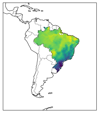
As a first example, we will select a geospatial extent defined by its longitudinal (W–E) and latitudinal (S–N) coverage.
ds_extent = egh.select_extent(ds, [-80, -10, 0, 30])  # W, E, S, N
ds_extent
<xarray.Dataset> Size: 6GB
Dimensions:  (time: 1008, cell: 2326, level: 37)
Coordinates:
  * time     (time) datetime64[ns] 8kB 1940-01-01 1940-02-01 ... 2023-12-01
  * cell     (cell) float32 9kB 1.229e+04 1.229e+04 ... 3.225e+04 3.226e+04
  * level    (level) float32 148B 1.0 2.0 3.0 5.0 ... 925.0 950.0 975.0 1e+03
    crs      float32 4B ...
    lat      (cell) float32 9kB dask.array<chunksize=(2326,), meta=np.ndarray>
    lon      (cell) float32 9kB dask.array<chunksize=(2326,), meta=np.ndarray>
Data variables: (12/111)
    100u     (time, cell) float32 9MB dask.array<chunksize=(24, 2326), meta=np.ndarray>
    100v     (time, cell) float32 9MB dask.array<chunksize=(24, 2326), meta=np.ndarray>
    10fg     (time, cell) float32 9MB dask.array<chunksize=(24, 2326), meta=np.ndarray>
    10si     (time, cell) float32 9MB dask.array<chunksize=(24, 2326), meta=np.ndarray>
    10u      (time, cell) float32 9MB dask.array<chunksize=(24, 2326), meta=np.ndarray>
    10v      (time, cell) float32 9MB dask.array<chunksize=(24, 2326), meta=np.ndarray>
    ...       ...
    uvb      (time, cell) float32 9MB dask.array<chunksize=(24, 2326), meta=np.ndarray>
    v        (time, level, cell) float32 347MB dask.array<chunksize=(24, 4, 2326), meta=np.ndarray>
    vo       (time, level, cell) float32 347MB dask.array<chunksize=(24, 4, 2326), meta=np.ndarray>
    w        (time, level, cell) float32 347MB dask.array<chunksize=(24, 4, 2326), meta=np.ndarray>
    z        (time, level, cell) float32 347MB dask.array<chunksize=(24, 4, 2326), meta=np.ndarray>
    zust     (time, cell) float32 9MB dask.array<chunksize=(24, 2326), meta=np.ndarray>
Attributes:
    acknowledgment:  Contains modified Copernicus Climate Change Service info...
    contact:         lukas.kluft@mpimet.mpg.de
    creator:         Lukas Kluft
    description:     HEALPixelation of ERA5
source: Post-processed dataset based on the ERA5 mirror located ...- time: 1008
- cell: 2326
- level: 37
- time(time)datetime64[ns]1940-01-01 ... 2023-12-01
- axis :
- T
array(['1940-01-01T00:00:00.000000000', '1940-02-01T00:00:00.000000000', '1940-03-01T00:00:00.000000000', ..., '2023-10-01T00:00:00.000000000', '2023-11-01T00:00:00.000000000', '2023-12-01T00:00:00.000000000'], shape=(1008,), dtype='datetime64[ns]') - cell(cell)float321.229e+04 1.229e+04 ... 3.226e+04
array([12288., 12289., 12290., ..., 32253., 32254., 32255.], shape=(2326,), dtype=float32) - level(level)float321.0 2.0 3.0 ... 950.0 975.0 1e+03
- axis :
- Z
- long_name :
- Air pressure at model level
- positive :
- down
- standard_name :
- air_pressure
- units :
- hPa
array([ 1., 2., 3., 5., 7., 10., 20., 30., 50., 70., 100., 125., 150., 175., 200., 225., 250., 300., 350., 400., 450., 500., 550., 600., 650., 700., 750., 775., 800., 825., 850., 875., 900., 925., 950., 975., 1000.], dtype=float32) - crs()float32...
- grid_mapping_name :
- healpix
- healpix_nside :
- 64
- healpix_order :
- nested
[1 values with dtype=float32]
- lat(cell)float32dask.array<chunksize=(2326,), meta=np.ndarray>
- long_name :
- latitude
- standard_name :
- latitude
- units :
- degrees_north
Array Chunk Bytes 9.09 kiB 9.09 kiB Shape (2326,) (2326,) Dask graph 1 chunks in 3 graph layers Data type float32 numpy.ndarray - lon(cell)float32dask.array<chunksize=(2326,), meta=np.ndarray>
- long_name :
- longitude
- standard_name :
- longitude
- units :
- degrees_east
Array Chunk Bytes 9.09 kiB 9.09 kiB Shape (2326,) (2326,) Dask graph 1 chunks in 3 graph layers Data type float32 numpy.ndarray
- 100u(time, cell)float32dask.array<chunksize=(24, 2326), meta=np.ndarray>
- grid_mapping :
- crs
- levtype :
- surface
- long_name :
- 100 metre U wind component
- standard_name :
- units :
- m s**-1
Array Chunk Bytes 8.94 MiB 218.06 kiB Shape (1008, 2326) (24, 2326) Dask graph 42 chunks in 3 graph layers Data type float32 numpy.ndarray - 100v(time, cell)float32dask.array<chunksize=(24, 2326), meta=np.ndarray>
- grid_mapping :
- crs
- levtype :
- surface
- long_name :
- 100 metre V wind component
- standard_name :
- units :
- m s**-1
Array Chunk Bytes 8.94 MiB 218.06 kiB Shape (1008, 2326) (24, 2326) Dask graph 42 chunks in 3 graph layers Data type float32 numpy.ndarray - 10fg(time, cell)float32dask.array<chunksize=(24, 2326), meta=np.ndarray>
- grid_mapping :
- crs
- levtype :
- surface
- long_name :
- 10 metre wind gust since previous post-processing
- standard_name :
- units :
- m s**-1
Array Chunk Bytes 8.94 MiB 218.06 kiB Shape (1008, 2326) (24, 2326) Dask graph 42 chunks in 3 graph layers Data type float32 numpy.ndarray - 10si(time, cell)float32dask.array<chunksize=(24, 2326), meta=np.ndarray>
- grid_mapping :
- crs
- levtype :
- surface
- long_name :
- 10 metre wind speed
- standard_name :
- units :
- m s**-1
Array Chunk Bytes 8.94 MiB 218.06 kiB Shape (1008, 2326) (24, 2326) Dask graph 42 chunks in 3 graph layers Data type float32 numpy.ndarray - 10u(time, cell)float32dask.array<chunksize=(24, 2326), meta=np.ndarray>
- grid_mapping :
- crs
- levtype :
- surface
- long_name :
- 10 metre U wind component
- standard_name :
- units :
- m s**-1
Array Chunk Bytes 8.94 MiB 218.06 kiB Shape (1008, 2326) (24, 2326) Dask graph 42 chunks in 3 graph layers Data type float32 numpy.ndarray - 10v(time, cell)float32dask.array<chunksize=(24, 2326), meta=np.ndarray>
- grid_mapping :
- crs
- levtype :
- surface
- long_name :
- 10 metre V wind component
- standard_name :
- units :
- m s**-1
Array Chunk Bytes 8.94 MiB 218.06 kiB Shape (1008, 2326) (24, 2326) Dask graph 42 chunks in 3 graph layers Data type float32 numpy.ndarray - 2d(time, cell)float32dask.array<chunksize=(24, 2326), meta=np.ndarray>
- grid_mapping :
- crs
- levtype :
- surface
- long_name :
- 2 metre dewpoint temperature
- standard_name :
- units :
- K
Array Chunk Bytes 8.94 MiB 218.06 kiB Shape (1008, 2326) (24, 2326) Dask graph 42 chunks in 3 graph layers Data type float32 numpy.ndarray - 2t(time, cell)float32dask.array<chunksize=(24, 2326), meta=np.ndarray>
- grid_mapping :
- crs
- levtype :
- surface
- long_name :
- 2 metre temperature
- standard_name :
- units :
- K
Array Chunk Bytes 8.94 MiB 218.06 kiB Shape (1008, 2326) (24, 2326) Dask graph 42 chunks in 3 graph layers Data type float32 numpy.ndarray - asn(time, cell)float32dask.array<chunksize=(24, 2326), meta=np.ndarray>
- grid_mapping :
- crs
- levtype :
- surface
- long_name :
- Snow albedo
- standard_name :
- units :
- (0 - 1)
Array Chunk Bytes 8.94 MiB 218.06 kiB Shape (1008, 2326) (24, 2326) Dask graph 42 chunks in 3 graph layers Data type float32 numpy.ndarray - bld(time, cell)float32dask.array<chunksize=(24, 2326), meta=np.ndarray>
- grid_mapping :
- crs
- levtype :
- surface
- long_name :
- Boundary layer dissipation
- standard_name :
- kinetic_energy_dissipation_in_atmosphere_boundary_layer
- units :
- J m**-2
Array Chunk Bytes 8.94 MiB 218.06 kiB Shape (1008, 2326) (24, 2326) Dask graph 42 chunks in 3 graph layers Data type float32 numpy.ndarray - blh(time, cell)float32dask.array<chunksize=(24, 2326), meta=np.ndarray>
- grid_mapping :
- crs
- levtype :
- surface
- long_name :
- Boundary layer height
- standard_name :
- units :
- m
Array Chunk Bytes 8.94 MiB 218.06 kiB Shape (1008, 2326) (24, 2326) Dask graph 42 chunks in 3 graph layers Data type float32 numpy.ndarray - cape(time, cell)float32dask.array<chunksize=(24, 2326), meta=np.ndarray>
- grid_mapping :
- crs
- levtype :
- surface
- long_name :
- Convective available potential energy
- standard_name :
- units :
- J kg**-1
Array Chunk Bytes 8.94 MiB 218.06 kiB Shape (1008, 2326) (24, 2326) Dask graph 42 chunks in 3 graph layers Data type float32 numpy.ndarray - cbh(time, cell)float32dask.array<chunksize=(24, 2326), meta=np.ndarray>
- grid_mapping :
- crs
- levtype :
- surface
- long_name :
- Cloud base height
- standard_name :
- units :
- m
Array Chunk Bytes 8.94 MiB 218.06 kiB Shape (1008, 2326) (24, 2326) Dask graph 42 chunks in 3 graph layers Data type float32 numpy.ndarray - cc(time, level, cell)float32dask.array<chunksize=(24, 4, 2326), meta=np.ndarray>
- grid_mapping :
- crs
- levtype :
- isobaricInhPa
- long_name :
- Fraction of cloud cover
- standard_name :
- units :
- (0 - 1)
Array Chunk Bytes 330.93 MiB 872.25 kiB Shape (1008, 37, 2326) (24, 4, 2326) Dask graph 420 chunks in 3 graph layers Data type float32 numpy.ndarray - cdir(time, cell)float32dask.array<chunksize=(24, 2326), meta=np.ndarray>
- grid_mapping :
- crs
- levtype :
- surface
- long_name :
- Clear-sky direct solar radiation at surface
- standard_name :
- units :
- J m**-2
Array Chunk Bytes 8.94 MiB 218.06 kiB Shape (1008, 2326) (24, 2326) Dask graph 42 chunks in 3 graph layers Data type float32 numpy.ndarray - ci(time, cell)float32dask.array<chunksize=(24, 2326), meta=np.ndarray>
- grid_mapping :
- crs
- levtype :
- surface
- long_name :
- Sea ice area fraction
- standard_name :
- sea_ice_area_fraction
- units :
- (0 - 1)
Array Chunk Bytes 8.94 MiB 218.06 kiB Shape (1008, 2326) (24, 2326) Dask graph 42 chunks in 3 graph layers Data type float32 numpy.ndarray - ciwc(time, level, cell)float32dask.array<chunksize=(24, 4, 2326), meta=np.ndarray>
- grid_mapping :
- crs
- levtype :
- isobaricInhPa
- long_name :
- Specific cloud ice water content
- standard_name :
- units :
- kg kg**-1
Array Chunk Bytes 330.93 MiB 872.25 kiB Shape (1008, 37, 2326) (24, 4, 2326) Dask graph 420 chunks in 3 graph layers Data type float32 numpy.ndarray - clwc(time, level, cell)float32dask.array<chunksize=(24, 4, 2326), meta=np.ndarray>
- grid_mapping :
- crs
- levtype :
- isobaricInhPa
- long_name :
- Specific cloud liquid water content
- standard_name :
- units :
- kg kg**-1
Array Chunk Bytes 330.93 MiB 872.25 kiB Shape (1008, 37, 2326) (24, 4, 2326) Dask graph 420 chunks in 3 graph layers Data type float32 numpy.ndarray - cp(time, cell)float32dask.array<chunksize=(24, 2326), meta=np.ndarray>
- grid_mapping :
- crs
- levtype :
- surface
- long_name :
- Convective precipitation
- standard_name :
- lwe_thickness_of_convective_precipitation_amount
- units :
- m
Array Chunk Bytes 8.94 MiB 218.06 kiB Shape (1008, 2326) (24, 2326) Dask graph 42 chunks in 3 graph layers Data type float32 numpy.ndarray - crr(time, cell)float32dask.array<chunksize=(24, 2326), meta=np.ndarray>
- grid_mapping :
- crs
- levtype :
- surface
- long_name :
- Convective rain rate
- standard_name :
- units :
- kg m**-2 s**-1
Array Chunk Bytes 8.94 MiB 218.06 kiB Shape (1008, 2326) (24, 2326) Dask graph 42 chunks in 3 graph layers Data type float32 numpy.ndarray - crwc(time, level, cell)float32dask.array<chunksize=(24, 4, 2326), meta=np.ndarray>
- grid_mapping :
- crs
- levtype :
- isobaricInhPa
- long_name :
- Specific rain water content
- standard_name :
- units :
- kg kg**-1
Array Chunk Bytes 330.93 MiB 872.25 kiB Shape (1008, 37, 2326) (24, 4, 2326) Dask graph 420 chunks in 3 graph layers Data type float32 numpy.ndarray - csf(time, cell)float32dask.array<chunksize=(24, 2326), meta=np.ndarray>
- grid_mapping :
- crs
- levtype :
- surface
- long_name :
- Convective snowfall
- standard_name :
- units :
- m of water equivalent
Array Chunk Bytes 8.94 MiB 218.06 kiB Shape (1008, 2326) (24, 2326) Dask graph 42 chunks in 3 graph layers Data type float32 numpy.ndarray - csfr(time, cell)float32dask.array<chunksize=(24, 2326), meta=np.ndarray>
- grid_mapping :
- crs
- levtype :
- surface
- long_name :
- Convective snowfall rate water equivalent
- standard_name :
- units :
- kg m**-2 s**-1
Array Chunk Bytes 8.94 MiB 218.06 kiB Shape (1008, 2326) (24, 2326) Dask graph 42 chunks in 3 graph layers Data type float32 numpy.ndarray - cswc(time, level, cell)float32dask.array<chunksize=(24, 4, 2326), meta=np.ndarray>
- grid_mapping :
- crs
- levtype :
- isobaricInhPa
- long_name :
- Specific snow water content
- standard_name :
- units :
- kg kg**-1
Array Chunk Bytes 330.93 MiB 872.25 kiB Shape (1008, 37, 2326) (24, 4, 2326) Dask graph 420 chunks in 3 graph layers Data type float32 numpy.ndarray - d(time, level, cell)float32dask.array<chunksize=(24, 4, 2326), meta=np.ndarray>
- grid_mapping :
- crs
- levtype :
- isobaricInhPa
- long_name :
- Divergence
- standard_name :
- divergence_of_wind
- units :
- s**-1
Array Chunk Bytes 330.93 MiB 872.25 kiB Shape (1008, 37, 2326) (24, 4, 2326) Dask graph 420 chunks in 3 graph layers Data type float32 numpy.ndarray - e(time, cell)float32dask.array<chunksize=(24, 2326), meta=np.ndarray>
- grid_mapping :
- crs
- levtype :
- surface
- long_name :
- Evaporation
- standard_name :
- lwe_thickness_of_water_evaporation_amount
- units :
- m of water equivalent
Array Chunk Bytes 8.94 MiB 218.06 kiB Shape (1008, 2326) (24, 2326) Dask graph 42 chunks in 3 graph layers Data type float32 numpy.ndarray - es(time, cell)float32dask.array<chunksize=(24, 2326), meta=np.ndarray>
- grid_mapping :
- crs
- levtype :
- surface
- long_name :
- Snow evaporation
- standard_name :
- units :
- m of water equivalent
Array Chunk Bytes 8.94 MiB 218.06 kiB Shape (1008, 2326) (24, 2326) Dask graph 42 chunks in 3 graph layers Data type float32 numpy.ndarray - ewss(time, cell)float32dask.array<chunksize=(24, 2326), meta=np.ndarray>
- grid_mapping :
- crs
- levtype :
- surface
- long_name :
- Eastward turbulent surface stress
- standard_name :
- surface_downward_eastward_stress
- units :
- N m**-2 s
Array Chunk Bytes 8.94 MiB 218.06 kiB Shape (1008, 2326) (24, 2326) Dask graph 42 chunks in 3 graph layers Data type float32 numpy.ndarray - fal(time, cell)float32dask.array<chunksize=(24, 2326), meta=np.ndarray>
- grid_mapping :
- crs
- levtype :
- surface
- long_name :
- Forecast albedo
- standard_name :
- units :
- (0 - 1)
Array Chunk Bytes 8.94 MiB 218.06 kiB Shape (1008, 2326) (24, 2326) Dask graph 42 chunks in 3 graph layers Data type float32 numpy.ndarray - fdir(time, cell)float32dask.array<chunksize=(24, 2326), meta=np.ndarray>
- grid_mapping :
- crs
- levtype :
- surface
- long_name :
- Total sky direct solar radiation at surface
- standard_name :
- units :
- J m**-2
Array Chunk Bytes 8.94 MiB 218.06 kiB Shape (1008, 2326) (24, 2326) Dask graph 42 chunks in 3 graph layers Data type float32 numpy.ndarray - flsr(time, cell)float32dask.array<chunksize=(24, 2326), meta=np.ndarray>
- grid_mapping :
- crs
- levtype :
- surface
- long_name :
- Forecast logarithm of surface roughness for heat
- standard_name :
- units :
- ~
Array Chunk Bytes 8.94 MiB 218.06 kiB Shape (1008, 2326) (24, 2326) Dask graph 42 chunks in 3 graph layers Data type float32 numpy.ndarray - fsr(time, cell)float32dask.array<chunksize=(24, 2326), meta=np.ndarray>
- grid_mapping :
- crs
- levtype :
- surface
- long_name :
- Forecast surface roughness
- standard_name :
- units :
- m
Array Chunk Bytes 8.94 MiB 218.06 kiB Shape (1008, 2326) (24, 2326) Dask graph 42 chunks in 3 graph layers Data type float32 numpy.ndarray - gwd(time, cell)float32dask.array<chunksize=(24, 2326), meta=np.ndarray>
- grid_mapping :
- crs
- levtype :
- surface
- long_name :
- Gravity wave dissipation
- standard_name :
- units :
- J m**-2
Array Chunk Bytes 8.94 MiB 218.06 kiB Shape (1008, 2326) (24, 2326) Dask graph 42 chunks in 3 graph layers Data type float32 numpy.ndarray - hcc(time, cell)float32dask.array<chunksize=(24, 2326), meta=np.ndarray>
- grid_mapping :
- crs
- levtype :
- surface
- long_name :
- High cloud cover
- standard_name :
- units :
- (0 - 1)
Array Chunk Bytes 8.94 MiB 218.06 kiB Shape (1008, 2326) (24, 2326) Dask graph 42 chunks in 3 graph layers Data type float32 numpy.ndarray - i10fg(time, cell)float32dask.array<chunksize=(24, 2326), meta=np.ndarray>
- grid_mapping :
- crs
- levtype :
- surface
- long_name :
- Instantaneous 10 metre wind gust
- standard_name :
- units :
- m s**-1
Array Chunk Bytes 8.94 MiB 218.06 kiB Shape (1008, 2326) (24, 2326) Dask graph 42 chunks in 3 graph layers Data type float32 numpy.ndarray - ie(time, cell)float32dask.array<chunksize=(24, 2326), meta=np.ndarray>
- grid_mapping :
- crs
- levtype :
- surface
- long_name :
- Instantaneous moisture flux
- standard_name :
- units :
- kg m**-2 s**-1
Array Chunk Bytes 8.94 MiB 218.06 kiB Shape (1008, 2326) (24, 2326) Dask graph 42 chunks in 3 graph layers Data type float32 numpy.ndarray - istl1(time, cell)float32dask.array<chunksize=(24, 2326), meta=np.ndarray>
- grid_mapping :
- crs
- levtype :
- depthBelowLandLayer
- long_name :
- Ice temperature layer 1
- standard_name :
- units :
- K
Array Chunk Bytes 8.94 MiB 218.06 kiB Shape (1008, 2326) (24, 2326) Dask graph 42 chunks in 3 graph layers Data type float32 numpy.ndarray - istl2(time, cell)float32dask.array<chunksize=(24, 2326), meta=np.ndarray>
- grid_mapping :
- crs
- levtype :
- depthBelowLandLayer
- long_name :
- Ice temperature layer 2
- standard_name :
- units :
- K
Array Chunk Bytes 8.94 MiB 218.06 kiB Shape (1008, 2326) (24, 2326) Dask graph 42 chunks in 3 graph layers Data type float32 numpy.ndarray - istl3(time, cell)float32dask.array<chunksize=(24, 2326), meta=np.ndarray>
- grid_mapping :
- crs
- levtype :
- depthBelowLandLayer
- long_name :
- Ice temperature layer 3
- standard_name :
- units :
- K
Array Chunk Bytes 8.94 MiB 218.06 kiB Shape (1008, 2326) (24, 2326) Dask graph 42 chunks in 3 graph layers Data type float32 numpy.ndarray - istl4(time, cell)float32dask.array<chunksize=(24, 2326), meta=np.ndarray>
- grid_mapping :
- crs
- levtype :
- depthBelowLandLayer
- long_name :
- Ice temperature layer 4
- standard_name :
- units :
- K
Array Chunk Bytes 8.94 MiB 218.06 kiB Shape (1008, 2326) (24, 2326) Dask graph 42 chunks in 3 graph layers Data type float32 numpy.ndarray - lai_hv(time, cell)float32dask.array<chunksize=(24, 2326), meta=np.ndarray>
- grid_mapping :
- crs
- levtype :
- surface
- long_name :
- Leaf area index, high vegetation
- standard_name :
- units :
- m**2 m**-2
Array Chunk Bytes 8.94 MiB 218.06 kiB Shape (1008, 2326) (24, 2326) Dask graph 42 chunks in 3 graph layers Data type float32 numpy.ndarray - lai_lv(time, cell)float32dask.array<chunksize=(24, 2326), meta=np.ndarray>
- grid_mapping :
- crs
- levtype :
- surface
- long_name :
- Leaf area index, low vegetation
- standard_name :
- units :
- m**2 m**-2
Array Chunk Bytes 8.94 MiB 218.06 kiB Shape (1008, 2326) (24, 2326) Dask graph 42 chunks in 3 graph layers Data type float32 numpy.ndarray - lcc(time, cell)float32dask.array<chunksize=(24, 2326), meta=np.ndarray>
- grid_mapping :
- crs
- levtype :
- surface
- long_name :
- Low cloud cover
- standard_name :
- units :
- (0 - 1)
Array Chunk Bytes 8.94 MiB 218.06 kiB Shape (1008, 2326) (24, 2326) Dask graph 42 chunks in 3 graph layers Data type float32 numpy.ndarray - lgws(time, cell)float32dask.array<chunksize=(24, 2326), meta=np.ndarray>
- grid_mapping :
- crs
- levtype :
- surface
- long_name :
- Eastward gravity wave surface stress
- standard_name :
- units :
- N m**-2 s
Array Chunk Bytes 8.94 MiB 218.06 kiB Shape (1008, 2326) (24, 2326) Dask graph 42 chunks in 3 graph layers Data type float32 numpy.ndarray - lsf(time, cell)float32dask.array<chunksize=(24, 2326), meta=np.ndarray>
- grid_mapping :
- crs
- levtype :
- surface
- long_name :
- Large-scale snowfall
- standard_name :
- units :
- m of water equivalent
Array Chunk Bytes 8.94 MiB 218.06 kiB Shape (1008, 2326) (24, 2326) Dask graph 42 chunks in 3 graph layers Data type float32 numpy.ndarray - lsp(time, cell)float32dask.array<chunksize=(24, 2326), meta=np.ndarray>
- grid_mapping :
- crs
- levtype :
- surface
- long_name :
- Large-scale precipitation
- standard_name :
- lwe_thickness_of_stratiform_precipitation_amount
- units :
- m
Array Chunk Bytes 8.94 MiB 218.06 kiB Shape (1008, 2326) (24, 2326) Dask graph 42 chunks in 3 graph layers Data type float32 numpy.ndarray - lspf(time, cell)float32dask.array<chunksize=(24, 2326), meta=np.ndarray>
- grid_mapping :
- crs
- levtype :
- surface
- long_name :
- Large-scale precipitation fraction
- standard_name :
- units :
- s
Array Chunk Bytes 8.94 MiB 218.06 kiB Shape (1008, 2326) (24, 2326) Dask graph 42 chunks in 3 graph layers Data type float32 numpy.ndarray - lsrr(time, cell)float32dask.array<chunksize=(24, 2326), meta=np.ndarray>
- grid_mapping :
- crs
- levtype :
- surface
- long_name :
- Large scale rain rate
- standard_name :
- units :
- kg m**-2 s**-1
Array Chunk Bytes 8.94 MiB 218.06 kiB Shape (1008, 2326) (24, 2326) Dask graph 42 chunks in 3 graph layers Data type float32 numpy.ndarray - lssfr(time, cell)float32dask.array<chunksize=(24, 2326), meta=np.ndarray>
- grid_mapping :
- crs
- levtype :
- surface
- long_name :
- Large scale snowfall rate water equivalent
- standard_name :
- units :
- kg m**-2 s**-1
Array Chunk Bytes 8.94 MiB 218.06 kiB Shape (1008, 2326) (24, 2326) Dask graph 42 chunks in 3 graph layers Data type float32 numpy.ndarray - mcc(time, cell)float32dask.array<chunksize=(24, 2326), meta=np.ndarray>
- grid_mapping :
- crs
- levtype :
- surface
- long_name :
- Medium cloud cover
- standard_name :
- units :
- (0 - 1)
Array Chunk Bytes 8.94 MiB 218.06 kiB Shape (1008, 2326) (24, 2326) Dask graph 42 chunks in 3 graph layers Data type float32 numpy.ndarray - mgws(time, cell)float32dask.array<chunksize=(24, 2326), meta=np.ndarray>
- grid_mapping :
- crs
- levtype :
- surface
- long_name :
- Northward gravity wave surface stress
- standard_name :
- units :
- N m**-2 s
Array Chunk Bytes 8.94 MiB 218.06 kiB Shape (1008, 2326) (24, 2326) Dask graph 42 chunks in 3 graph layers Data type float32 numpy.ndarray - mn2t(time, cell)float32dask.array<chunksize=(24, 2326), meta=np.ndarray>
- grid_mapping :
- crs
- levtype :
- surface
- long_name :
- Minimum temperature at 2 metres since previous post-processing
- standard_name :
- units :
- K
Array Chunk Bytes 8.94 MiB 218.06 kiB Shape (1008, 2326) (24, 2326) Dask graph 42 chunks in 3 graph layers Data type float32 numpy.ndarray - msl(time, cell)float32dask.array<chunksize=(24, 2326), meta=np.ndarray>
- grid_mapping :
- crs
- levtype :
- surface
- long_name :
- Mean sea level pressure
- standard_name :
- air_pressure_at_mean_sea_level
- units :
- Pa
Array Chunk Bytes 8.94 MiB 218.06 kiB Shape (1008, 2326) (24, 2326) Dask graph 42 chunks in 3 graph layers Data type float32 numpy.ndarray - mx2t(time, cell)float32dask.array<chunksize=(24, 2326), meta=np.ndarray>
- grid_mapping :
- crs
- levtype :
- surface
- long_name :
- Maximum temperature at 2 metres since previous post-processing
- standard_name :
- units :
- K
Array Chunk Bytes 8.94 MiB 218.06 kiB Shape (1008, 2326) (24, 2326) Dask graph 42 chunks in 3 graph layers Data type float32 numpy.ndarray - nsss(time, cell)float32dask.array<chunksize=(24, 2326), meta=np.ndarray>
- grid_mapping :
- crs
- levtype :
- surface
- long_name :
- Northward turbulent surface stress
- standard_name :
- surface_downward_northward_stress
- units :
- N m**-2 s
Array Chunk Bytes 8.94 MiB 218.06 kiB Shape (1008, 2326) (24, 2326) Dask graph 42 chunks in 3 graph layers Data type float32 numpy.ndarray - o3(time, level, cell)float32dask.array<chunksize=(24, 4, 2326), meta=np.ndarray>
- grid_mapping :
- crs
- levtype :
- isobaricInhPa
- long_name :
- Ozone mass mixing ratio
- standard_name :
- mass_fraction_of_ozone_in_air
- units :
- kg kg**-1
Array Chunk Bytes 330.93 MiB 872.25 kiB Shape (1008, 37, 2326) (24, 4, 2326) Dask graph 420 chunks in 3 graph layers Data type float32 numpy.ndarray - pev(time, cell)float32dask.array<chunksize=(24, 2326), meta=np.ndarray>
- grid_mapping :
- crs
- levtype :
- surface
- long_name :
- Potential evaporation
- standard_name :
- units :
- m
Array Chunk Bytes 8.94 MiB 218.06 kiB Shape (1008, 2326) (24, 2326) Dask graph 42 chunks in 3 graph layers Data type float32 numpy.ndarray - pv(time, level, cell)float32dask.array<chunksize=(24, 4, 2326), meta=np.ndarray>
- grid_mapping :
- crs
- levtype :
- isobaricInhPa
- long_name :
- Potential vorticity
- standard_name :
- units :
- K m**2 kg**-1 s**-1
Array Chunk Bytes 330.93 MiB 872.25 kiB Shape (1008, 37, 2326) (24, 4, 2326) Dask graph 420 chunks in 3 graph layers Data type float32 numpy.ndarray - q(time, level, cell)float32dask.array<chunksize=(24, 4, 2326), meta=np.ndarray>
- grid_mapping :
- crs
- levtype :
- isobaricInhPa
- long_name :
- Specific humidity
- standard_name :
- specific_humidity
- units :
- kg kg**-1
Array Chunk Bytes 330.93 MiB 872.25 kiB Shape (1008, 37, 2326) (24, 4, 2326) Dask graph 420 chunks in 3 graph layers Data type float32 numpy.ndarray - r(time, level, cell)float32dask.array<chunksize=(24, 4, 2326), meta=np.ndarray>
- grid_mapping :
- crs
- levtype :
- isobaricInhPa
- long_name :
- Relative humidity
- standard_name :
- relative_humidity
- units :
- %
Array Chunk Bytes 330.93 MiB 872.25 kiB Shape (1008, 37, 2326) (24, 4, 2326) Dask graph 420 chunks in 3 graph layers Data type float32 numpy.ndarray - ro(time, cell)float32dask.array<chunksize=(24, 2326), meta=np.ndarray>
- grid_mapping :
- crs
- levtype :
- surface
- long_name :
- Runoff
- standard_name :
- units :
- m
Array Chunk Bytes 8.94 MiB 218.06 kiB Shape (1008, 2326) (24, 2326) Dask graph 42 chunks in 3 graph layers Data type float32 numpy.ndarray - rsn(time, cell)float32dask.array<chunksize=(24, 2326), meta=np.ndarray>
- grid_mapping :
- crs
- levtype :
- surface
- long_name :
- Snow density
- standard_name :
- units :
- kg m**-3
Array Chunk Bytes 8.94 MiB 218.06 kiB Shape (1008, 2326) (24, 2326) Dask graph 42 chunks in 3 graph layers Data type float32 numpy.ndarray - sd(time, cell)float32dask.array<chunksize=(24, 2326), meta=np.ndarray>
- grid_mapping :
- crs
- levtype :
- surface
- long_name :
- Snow depth
- standard_name :
- lwe_thickness_of_surface_snow_amount
- units :
- m of water equivalent
Array Chunk Bytes 8.94 MiB 218.06 kiB Shape (1008, 2326) (24, 2326) Dask graph 42 chunks in 3 graph layers Data type float32 numpy.ndarray - sf(time, cell)float32dask.array<chunksize=(24, 2326), meta=np.ndarray>
- grid_mapping :
- crs
- levtype :
- surface
- long_name :
- Snowfall
- standard_name :
- lwe_thickness_of_snowfall_amount
- units :
- m of water equivalent
Array Chunk Bytes 8.94 MiB 218.06 kiB Shape (1008, 2326) (24, 2326) Dask graph 42 chunks in 3 graph layers Data type float32 numpy.ndarray - skt(time, cell)float32dask.array<chunksize=(24, 2326), meta=np.ndarray>
- grid_mapping :
- crs
- levtype :
- surface
- long_name :
- Skin temperature
- standard_name :
- units :
- K
Array Chunk Bytes 8.94 MiB 218.06 kiB Shape (1008, 2326) (24, 2326) Dask graph 42 chunks in 3 graph layers Data type float32 numpy.ndarray - slhf(time, cell)float32dask.array<chunksize=(24, 2326), meta=np.ndarray>
- grid_mapping :
- crs
- levtype :
- surface
- long_name :
- Surface latent heat flux
- standard_name :
- surface_upward_latent_heat_flux
- units :
- J m**-2
Array Chunk Bytes 8.94 MiB 218.06 kiB Shape (1008, 2326) (24, 2326) Dask graph 42 chunks in 3 graph layers Data type float32 numpy.ndarray - smlt(time, cell)float32dask.array<chunksize=(24, 2326), meta=np.ndarray>
- grid_mapping :
- crs
- levtype :
- surface
- long_name :
- Snowmelt
- standard_name :
- units :
- m of water equivalent
Array Chunk Bytes 8.94 MiB 218.06 kiB Shape (1008, 2326) (24, 2326) Dask graph 42 chunks in 3 graph layers Data type float32 numpy.ndarray - sp(time, cell)float32dask.array<chunksize=(24, 2326), meta=np.ndarray>
- grid_mapping :
- crs
- levtype :
- surface
- long_name :
- Surface pressure
- standard_name :
- surface_air_pressure
- units :
- Pa
Array Chunk Bytes 8.94 MiB 218.06 kiB Shape (1008, 2326) (24, 2326) Dask graph 42 chunks in 3 graph layers Data type float32 numpy.ndarray - src(time, cell)float32dask.array<chunksize=(24, 2326), meta=np.ndarray>
- grid_mapping :
- crs
- levtype :
- surface
- long_name :
- Skin reservoir content
- standard_name :
- units :
- m of water equivalent
Array Chunk Bytes 8.94 MiB 218.06 kiB Shape (1008, 2326) (24, 2326) Dask graph 42 chunks in 3 graph layers Data type float32 numpy.ndarray - sro(time, cell)float32dask.array<chunksize=(24, 2326), meta=np.ndarray>
- grid_mapping :
- crs
- levtype :
- surface
- long_name :
- Surface runoff
- standard_name :
- units :
- m
Array Chunk Bytes 8.94 MiB 218.06 kiB Shape (1008, 2326) (24, 2326) Dask graph 42 chunks in 3 graph layers Data type float32 numpy.ndarray - sshf(time, cell)float32dask.array<chunksize=(24, 2326), meta=np.ndarray>
- grid_mapping :
- crs
- levtype :
- surface
- long_name :
- Surface sensible heat flux
- standard_name :
- surface_upward_sensible_heat_flux
- units :
- J m**-2
Array Chunk Bytes 8.94 MiB 218.06 kiB Shape (1008, 2326) (24, 2326) Dask graph 42 chunks in 3 graph layers Data type float32 numpy.ndarray - ssr(time, cell)float32dask.array<chunksize=(24, 2326), meta=np.ndarray>
- grid_mapping :
- crs
- levtype :
- surface
- long_name :
- Surface net short-wave (solar) radiation
- standard_name :
- surface_net_downward_shortwave_flux
- units :
- J m**-2
Array Chunk Bytes 8.94 MiB 218.06 kiB Shape (1008, 2326) (24, 2326) Dask graph 42 chunks in 3 graph layers Data type float32 numpy.ndarray - ssrc(time, cell)float32dask.array<chunksize=(24, 2326), meta=np.ndarray>
- grid_mapping :
- crs
- levtype :
- surface
- long_name :
- Surface net short-wave (solar) radiation, clear sky
- standard_name :
- surface_net_downward_shortwave_flux_assuming_clear_sky
- units :
- J m**-2
Array Chunk Bytes 8.94 MiB 218.06 kiB Shape (1008, 2326) (24, 2326) Dask graph 42 chunks in 3 graph layers Data type float32 numpy.ndarray - ssrd(time, cell)float32dask.array<chunksize=(24, 2326), meta=np.ndarray>
- grid_mapping :
- crs
- levtype :
- surface
- long_name :
- Surface short-wave (solar) radiation downwards
- standard_name :
- surface_downwelling_shortwave_flux_in_air
- units :
- J m**-2
Array Chunk Bytes 8.94 MiB 218.06 kiB Shape (1008, 2326) (24, 2326) Dask graph 42 chunks in 3 graph layers Data type float32 numpy.ndarray - ssrdc(time, cell)float32dask.array<chunksize=(24, 2326), meta=np.ndarray>
- grid_mapping :
- crs
- levtype :
- surface
- long_name :
- Surface solar radiation downward clear-sky
- standard_name :
- units :
- J m**-2
Array Chunk Bytes 8.94 MiB 218.06 kiB Shape (1008, 2326) (24, 2326) Dask graph 42 chunks in 3 graph layers Data type float32 numpy.ndarray - sst(time, cell)float32dask.array<chunksize=(24, 2326), meta=np.ndarray>
- grid_mapping :
- crs
- levtype :
- surface
- long_name :
- Sea surface temperature
- standard_name :
- units :
- K
Array Chunk Bytes 8.94 MiB 218.06 kiB Shape (1008, 2326) (24, 2326) Dask graph 42 chunks in 3 graph layers Data type float32 numpy.ndarray - stl1(time, cell)float32dask.array<chunksize=(24, 2326), meta=np.ndarray>
- grid_mapping :
- crs
- levtype :
- depthBelowLandLayer
- long_name :
- Soil temperature level 1
- standard_name :
- surface_temperature
- units :
- K
Array Chunk Bytes 8.94 MiB 218.06 kiB Shape (1008, 2326) (24, 2326) Dask graph 42 chunks in 3 graph layers Data type float32 numpy.ndarray - stl2(time, cell)float32dask.array<chunksize=(24, 2326), meta=np.ndarray>
- grid_mapping :
- crs
- levtype :
- depthBelowLandLayer
- long_name :
- Soil temperature level 2
- standard_name :
- units :
- K
Array Chunk Bytes 8.94 MiB 218.06 kiB Shape (1008, 2326) (24, 2326) Dask graph 42 chunks in 3 graph layers Data type float32 numpy.ndarray - stl3(time, cell)float32dask.array<chunksize=(24, 2326), meta=np.ndarray>
- grid_mapping :
- crs
- levtype :
- depthBelowLandLayer
- long_name :
- Soil temperature level 3
- standard_name :
- units :
- K
Array Chunk Bytes 8.94 MiB 218.06 kiB Shape (1008, 2326) (24, 2326) Dask graph 42 chunks in 3 graph layers Data type float32 numpy.ndarray - stl4(time, cell)float32dask.array<chunksize=(24, 2326), meta=np.ndarray>
- grid_mapping :
- crs
- levtype :
- depthBelowLandLayer
- long_name :
- Soil temperature level 4
- standard_name :
- units :
- K
Array Chunk Bytes 8.94 MiB 218.06 kiB Shape (1008, 2326) (24, 2326) Dask graph 42 chunks in 3 graph layers Data type float32 numpy.ndarray - str(time, cell)float32dask.array<chunksize=(24, 2326), meta=np.ndarray>
- grid_mapping :
- crs
- levtype :
- surface
- long_name :
- Surface net long-wave (thermal) radiation
- standard_name :
- surface_net_upward_longwave_flux
- units :
- J m**-2
Array Chunk Bytes 8.94 MiB 218.06 kiB Shape (1008, 2326) (24, 2326) Dask graph 42 chunks in 3 graph layers Data type float32 numpy.ndarray - strc(time, cell)float32dask.array<chunksize=(24, 2326), meta=np.ndarray>
- grid_mapping :
- crs
- levtype :
- surface
- long_name :
- Surface net long-wave (thermal) radiation, clear sky
- standard_name :
- surface_net_downward_longwave_flux_assuming_clear_sky
- units :
- J m**-2
Array Chunk Bytes 8.94 MiB 218.06 kiB Shape (1008, 2326) (24, 2326) Dask graph 42 chunks in 3 graph layers Data type float32 numpy.ndarray - strd(time, cell)float32dask.array<chunksize=(24, 2326), meta=np.ndarray>
- grid_mapping :
- crs
- levtype :
- surface
- long_name :
- Surface long-wave (thermal) radiation downwards
- standard_name :
- units :
- J m**-2
Array Chunk Bytes 8.94 MiB 218.06 kiB Shape (1008, 2326) (24, 2326) Dask graph 42 chunks in 3 graph layers Data type float32 numpy.ndarray - strdc(time, cell)float32dask.array<chunksize=(24, 2326), meta=np.ndarray>
- grid_mapping :
- crs
- levtype :
- surface
- long_name :
- Surface thermal radiation downward clear-sky
- standard_name :
- units :
- J m**-2
Array Chunk Bytes 8.94 MiB 218.06 kiB Shape (1008, 2326) (24, 2326) Dask graph 42 chunks in 3 graph layers Data type float32 numpy.ndarray - swvl1(time, cell)float32dask.array<chunksize=(24, 2326), meta=np.ndarray>
- grid_mapping :
- crs
- levtype :
- depthBelowLandLayer
- long_name :
- Volumetric soil water layer 1
- standard_name :
- units :
- m**3 m**-3
Array Chunk Bytes 8.94 MiB 218.06 kiB Shape (1008, 2326) (24, 2326) Dask graph 42 chunks in 3 graph layers Data type float32 numpy.ndarray - swvl2(time, cell)float32dask.array<chunksize=(24, 2326), meta=np.ndarray>
- grid_mapping :
- crs
- levtype :
- depthBelowLandLayer
- long_name :
- Volumetric soil water layer 2
- standard_name :
- units :
- m**3 m**-3
Array Chunk Bytes 8.94 MiB 218.06 kiB Shape (1008, 2326) (24, 2326) Dask graph 42 chunks in 3 graph layers Data type float32 numpy.ndarray - swvl3(time, cell)float32dask.array<chunksize=(24, 2326), meta=np.ndarray>
- grid_mapping :
- crs
- levtype :
- depthBelowLandLayer
- long_name :
- Volumetric soil water layer 3
- standard_name :
- units :
- m**3 m**-3
Array Chunk Bytes 8.94 MiB 218.06 kiB Shape (1008, 2326) (24, 2326) Dask graph 42 chunks in 3 graph layers Data type float32 numpy.ndarray - swvl4(time, cell)float32dask.array<chunksize=(24, 2326), meta=np.ndarray>
- grid_mapping :
- crs
- levtype :
- depthBelowLandLayer
- long_name :
- Volumetric soil water layer 4
- standard_name :
- units :
- m**3 m**-3
Array Chunk Bytes 8.94 MiB 218.06 kiB Shape (1008, 2326) (24, 2326) Dask graph 42 chunks in 3 graph layers Data type float32 numpy.ndarray - t(time, level, cell)float32dask.array<chunksize=(24, 4, 2326), meta=np.ndarray>
- grid_mapping :
- crs
- levtype :
- isobaricInhPa
- long_name :
- Temperature
- standard_name :
- air_temperature
- units :
- K
Array Chunk Bytes 330.93 MiB 872.25 kiB Shape (1008, 37, 2326) (24, 4, 2326) Dask graph 420 chunks in 3 graph layers Data type float32 numpy.ndarray - tcc(time, cell)float32dask.array<chunksize=(24, 2326), meta=np.ndarray>
- grid_mapping :
- crs
- levtype :
- surface
- long_name :
- Total cloud cover
- standard_name :
- cloud_area_fraction
- units :
- (0 - 1)
Array Chunk Bytes 8.94 MiB 218.06 kiB Shape (1008, 2326) (24, 2326) Dask graph 42 chunks in 3 graph layers Data type float32 numpy.ndarray - tciw(time, cell)float32dask.array<chunksize=(24, 2326), meta=np.ndarray>
- grid_mapping :
- crs
- levtype :
- surface
- long_name :
- Total column cloud ice water
- standard_name :
- units :
- kg m**-2
Array Chunk Bytes 8.94 MiB 218.06 kiB Shape (1008, 2326) (24, 2326) Dask graph 42 chunks in 3 graph layers Data type float32 numpy.ndarray - tclw(time, cell)float32dask.array<chunksize=(24, 2326), meta=np.ndarray>
- grid_mapping :
- crs
- levtype :
- surface
- long_name :
- Total column cloud liquid water
- standard_name :
- units :
- kg m**-2
Array Chunk Bytes 8.94 MiB 218.06 kiB Shape (1008, 2326) (24, 2326) Dask graph 42 chunks in 3 graph layers Data type float32 numpy.ndarray - tco3(time, cell)float32dask.array<chunksize=(24, 2326), meta=np.ndarray>
- grid_mapping :
- crs
- levtype :
- surface
- long_name :
- Total column ozone
- standard_name :
- atmosphere_mass_content_of_ozone
- units :
- kg m**-2
Array Chunk Bytes 8.94 MiB 218.06 kiB Shape (1008, 2326) (24, 2326) Dask graph 42 chunks in 3 graph layers Data type float32 numpy.ndarray - tcrw(time, cell)float32dask.array<chunksize=(24, 2326), meta=np.ndarray>
- grid_mapping :
- crs
- levtype :
- surface
- long_name :
- Total column rain water
- standard_name :
- units :
- kg m**-2
Array Chunk Bytes 8.94 MiB 218.06 kiB Shape (1008, 2326) (24, 2326) Dask graph 42 chunks in 3 graph layers Data type float32 numpy.ndarray - tcsw(time, cell)float32dask.array<chunksize=(24, 2326), meta=np.ndarray>
- grid_mapping :
- crs
- levtype :
- surface
- long_name :
- Total column snow water
- standard_name :
- units :
- kg m**-2
Array Chunk Bytes 8.94 MiB 218.06 kiB Shape (1008, 2326) (24, 2326) Dask graph 42 chunks in 3 graph layers Data type float32 numpy.ndarray - tcw(time, cell)float32dask.array<chunksize=(24, 2326), meta=np.ndarray>
- grid_mapping :
- crs
- levtype :
- surface
- long_name :
- Total column water
- standard_name :
- units :
- kg m**-2
Array Chunk Bytes 8.94 MiB 218.06 kiB Shape (1008, 2326) (24, 2326) Dask graph 42 chunks in 3 graph layers Data type float32 numpy.ndarray - tcwv(time, cell)float32dask.array<chunksize=(24, 2326), meta=np.ndarray>
- grid_mapping :
- crs
- levtype :
- surface
- long_name :
- Total column vertically-integrated water vapour
- standard_name :
- lwe_thickness_of_atmosphere_mass_content_of_water_vapor
- units :
- kg m**-2
Array Chunk Bytes 8.94 MiB 218.06 kiB Shape (1008, 2326) (24, 2326) Dask graph 42 chunks in 3 graph layers Data type float32 numpy.ndarray - tisr(time, cell)float32dask.array<chunksize=(24, 2326), meta=np.ndarray>
- grid_mapping :
- crs
- levtype :
- surface
- long_name :
- TOA incident solar radiation
- standard_name :
- units :
- J m**-2
Array Chunk Bytes 8.94 MiB 218.06 kiB Shape (1008, 2326) (24, 2326) Dask graph 42 chunks in 3 graph layers Data type float32 numpy.ndarray - tp(time, cell)float32dask.array<chunksize=(24, 2326), meta=np.ndarray>
- grid_mapping :
- crs
- levtype :
- surface
- long_name :
- Total precipitation
- standard_name :
- units :
- m
Array Chunk Bytes 8.94 MiB 218.06 kiB Shape (1008, 2326) (24, 2326) Dask graph 42 chunks in 3 graph layers Data type float32 numpy.ndarray - tsn(time, cell)float32dask.array<chunksize=(24, 2326), meta=np.ndarray>
- grid_mapping :
- crs
- levtype :
- surface
- long_name :
- Temperature of snow layer
- standard_name :
- temperature_in_surface_snow
- units :
- K
Array Chunk Bytes 8.94 MiB 218.06 kiB Shape (1008, 2326) (24, 2326) Dask graph 42 chunks in 3 graph layers Data type float32 numpy.ndarray - tsr(time, cell)float32dask.array<chunksize=(24, 2326), meta=np.ndarray>
- grid_mapping :
- crs
- levtype :
- surface
- long_name :
- Top net short-wave (solar) radiation
- standard_name :
- toa_net_upward_shortwave_flux
- units :
- J m**-2
Array Chunk Bytes 8.94 MiB 218.06 kiB Shape (1008, 2326) (24, 2326) Dask graph 42 chunks in 3 graph layers Data type float32 numpy.ndarray - tsrc(time, cell)float32dask.array<chunksize=(24, 2326), meta=np.ndarray>
- grid_mapping :
- crs
- levtype :
- surface
- long_name :
- Top net solar radiation, clear sky
- standard_name :
- units :
- J m**-2
Array Chunk Bytes 8.94 MiB 218.06 kiB Shape (1008, 2326) (24, 2326) Dask graph 42 chunks in 3 graph layers Data type float32 numpy.ndarray - ttr(time, cell)float32dask.array<chunksize=(24, 2326), meta=np.ndarray>
- grid_mapping :
- crs
- levtype :
- surface
- long_name :
- Top net long-wave (thermal) radiation
- standard_name :
- toa_outgoing_longwave_flux
- units :
- J m**-2
Array Chunk Bytes 8.94 MiB 218.06 kiB Shape (1008, 2326) (24, 2326) Dask graph 42 chunks in 3 graph layers Data type float32 numpy.ndarray - ttrc(time, cell)float32dask.array<chunksize=(24, 2326), meta=np.ndarray>
- grid_mapping :
- crs
- levtype :
- surface
- long_name :
- Top net thermal radiation, clear sky
- standard_name :
- units :
- J m**-2
Array Chunk Bytes 8.94 MiB 218.06 kiB Shape (1008, 2326) (24, 2326) Dask graph 42 chunks in 3 graph layers Data type float32 numpy.ndarray - u(time, level, cell)float32dask.array<chunksize=(24, 4, 2326), meta=np.ndarray>
- grid_mapping :
- crs
- levtype :
- isobaricInhPa
- long_name :
- U component of wind
- standard_name :
- eastward_wind
- units :
- m s**-1
Array Chunk Bytes 330.93 MiB 872.25 kiB Shape (1008, 37, 2326) (24, 4, 2326) Dask graph 420 chunks in 3 graph layers Data type float32 numpy.ndarray - uvb(time, cell)float32dask.array<chunksize=(24, 2326), meta=np.ndarray>
- grid_mapping :
- crs
- levtype :
- surface
- long_name :
- Downward UV radiation at the surface
- standard_name :
- units :
- J m**-2
Array Chunk Bytes 8.94 MiB 218.06 kiB Shape (1008, 2326) (24, 2326) Dask graph 42 chunks in 3 graph layers Data type float32 numpy.ndarray - v(time, level, cell)float32dask.array<chunksize=(24, 4, 2326), meta=np.ndarray>
- grid_mapping :
- crs
- levtype :
- isobaricInhPa
- long_name :
- V component of wind
- standard_name :
- northward_wind
- units :
- m s**-1
Array Chunk Bytes 330.93 MiB 872.25 kiB Shape (1008, 37, 2326) (24, 4, 2326) Dask graph 420 chunks in 3 graph layers Data type float32 numpy.ndarray - vo(time, level, cell)float32dask.array<chunksize=(24, 4, 2326), meta=np.ndarray>
- grid_mapping :
- crs
- levtype :
- isobaricInhPa
- long_name :
- Vorticity (relative)
- standard_name :
- atmosphere_relative_vorticity
- units :
- s**-1
Array Chunk Bytes 330.93 MiB 872.25 kiB Shape (1008, 37, 2326) (24, 4, 2326) Dask graph 420 chunks in 3 graph layers Data type float32 numpy.ndarray - w(time, level, cell)float32dask.array<chunksize=(24, 4, 2326), meta=np.ndarray>
- grid_mapping :
- crs
- levtype :
- isobaricInhPa
- long_name :
- Vertical velocity
- standard_name :
- lagrangian_tendency_of_air_pressure
- units :
- Pa s**-1
Array Chunk Bytes 330.93 MiB 872.25 kiB Shape (1008, 37, 2326) (24, 4, 2326) Dask graph 420 chunks in 3 graph layers Data type float32 numpy.ndarray - z(time, level, cell)float32dask.array<chunksize=(24, 4, 2326), meta=np.ndarray>
- grid_mapping :
- crs
- levtype :
- isobaricInhPa
- long_name :
- Geopotential
- standard_name :
- geopotential
- units :
- m**2 s**-2
Array Chunk Bytes 330.93 MiB 872.25 kiB Shape (1008, 37, 2326) (24, 4, 2326) Dask graph 420 chunks in 3 graph layers Data type float32 numpy.ndarray - zust(time, cell)float32dask.array<chunksize=(24, 2326), meta=np.ndarray>
- grid_mapping :
- crs
- levtype :
- surface
- long_name :
- Friction velocity
- standard_name :
- units :
- m s**-1
Array Chunk Bytes 8.94 MiB 218.06 kiB Shape (1008, 2326) (24, 2326) Dask graph 42 chunks in 3 graph layers Data type float32 numpy.ndarray
- acknowledgment :
- Contains modified Copernicus Climate Change Service information 2020. Neither the European Commission nor ECMWF is responsible for any use that may be made of the Copernicus information or data it contains.
- contact :
- lukas.kluft@mpimet.mpg.de
- creator :
- Lukas Kluft
- description :
- HEALPixelation of ERA5
- source :
- Post-processed dataset based on the ERA5 mirror located at DKRZ.
egh.healpix_show(ds_extent["2t"].sel(time="2020-02-01"))
<matplotlib.image.AxesImage at 0x7f9df2401be0>
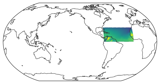
Geodesic section#
Next, we will select a geospatial section defined by a start point (lon1, lat1) and an end point (lon2, lat2).
The returned dataset is still ordered as the original global HEALPix map.
Since HEALPix indices do not follow a simple geospatial order, sorting by a coordinate such as lat makes the data easier to work with for plotting or further analysis.
ds_section = egh.select_section(ds, 10, -60, -60, 60).sortby("lat")
ds_section
<xarray.Dataset> Size: 499MB
Dimensions:  (time: 1008, cell: 180, level: 37)
Coordinates:
  * time     (time) datetime64[ns] 8kB 1940-01-01 1940-02-01 ... 2023-12-01
  * cell     (cell) float32 720B 3.486e+04 3.486e+04 ... 1.589e+04 1.59e+04
  * level    (level) float32 148B 1.0 2.0 3.0 5.0 ... 925.0 950.0 975.0 1e+03
    crs      float32 4B ...
    lat      (cell) float32 720B dask.array<chunksize=(180,), meta=np.ndarray>
    lon      (cell) float32 720B dask.array<chunksize=(180,), meta=np.ndarray>
Data variables: (12/111)
    100u     (time, cell) float32 726kB dask.array<chunksize=(24, 180), meta=np.ndarray>
    100v     (time, cell) float32 726kB dask.array<chunksize=(24, 180), meta=np.ndarray>
    10fg     (time, cell) float32 726kB dask.array<chunksize=(24, 180), meta=np.ndarray>
    10si     (time, cell) float32 726kB dask.array<chunksize=(24, 180), meta=np.ndarray>
    10u      (time, cell) float32 726kB dask.array<chunksize=(24, 180), meta=np.ndarray>
    10v      (time, cell) float32 726kB dask.array<chunksize=(24, 180), meta=np.ndarray>
    ...       ...
    uvb      (time, cell) float32 726kB dask.array<chunksize=(24, 180), meta=np.ndarray>
    v        (time, level, cell) float32 27MB dask.array<chunksize=(24, 4, 180), meta=np.ndarray>
    vo       (time, level, cell) float32 27MB dask.array<chunksize=(24, 4, 180), meta=np.ndarray>
    w        (time, level, cell) float32 27MB dask.array<chunksize=(24, 4, 180), meta=np.ndarray>
    z        (time, level, cell) float32 27MB dask.array<chunksize=(24, 4, 180), meta=np.ndarray>
    zust     (time, cell) float32 726kB dask.array<chunksize=(24, 180), meta=np.ndarray>
Attributes:
    acknowledgment:  Contains modified Copernicus Climate Change Service info...
    contact:         lukas.kluft@mpimet.mpg.de
    creator:         Lukas Kluft
    description:     HEALPixelation of ERA5
source: Post-processed dataset based on the ERA5 mirror located ...- time: 1008
- cell: 180
- level: 37
- time(time)datetime64[ns]1940-01-01 ... 2023-12-01
- axis :
- T
array(['1940-01-01T00:00:00.000000000', '1940-02-01T00:00:00.000000000', '1940-03-01T00:00:00.000000000', ..., '2023-10-01T00:00:00.000000000', '2023-11-01T00:00:00.000000000', '2023-12-01T00:00:00.000000000'], shape=(1008,), dtype='datetime64[ns]') - cell(cell)float323.486e+04 3.486e+04 ... 1.59e+04
array([34855., 34864., 34861., 34866., 34863., 34949., 34950., 34951., 34956., 34958., 34977., 34979., 34980., 34985., 34986., 34987., 35328., 35330., 35336., 35338., 46341., 46352., 46354., 46355., 46361., 46364., 46365., 46367., 46410., 46432., 46433., 46435., 46438., 46444., 46446., 46532., 46533., 46535., 46541., 46543., 46576., 46578., 46584., 46586., 46587., 46929., 46931., 46934., 46940., 46942., 46964., 46965., 46967., 46973., 16936., 16938., 17024., 17025., 17027., 17033., 17036., 17038., 17060., 17063., 17069., 17082., 18448., 18449., 18451., 18457., 18460., 18462., 18484., 18485., 18487., 18493., 18536., 18538., 18624., 18625., 18627., 18633., 18636., 18638., 18660., 18661., 18663., 18674., 18680., 18682., 18683., 19025., 19027., 19030., 19036., 19038., 19039., 19061., 19232., 19234., 19240., 19241., 19243., 19329., 19332., 19334., 19340., 19341., 19343., 19365., 19376., 19378., 19385., 19387., 19390., 12564., 12566., 12567., 12573., 12575., 12618., 12640., 12642., 12643., 12649., 12651., 12654., 12740., 12742., 12743., 12749., 12751., 12762., 12784., 12786., 12792., 12793., 12795., 13137., 13140., 13142., 13148., 13150., 13151., 13173., 13175., 13181., 13864., 13866., 13952., 13954., 13955., 13961., 13963., 13985., 13987., 13993., 13996., 13998., 15364., 15366., 15372., 15374., 15396., 15398., 15399., 15405., 15407., 15493., 15495., 15501., 15503., 15514., 15536., 15538., 15544., 15546., 15888., 15890., 15896.], dtype=float32) - level(level)float321.0 2.0 3.0 ... 950.0 975.0 1e+03
- axis :
- Z
- long_name :
- Air pressure at model level
- positive :
- down
- standard_name :
- air_pressure
- units :
- hPa
array([ 1., 2., 3., 5., 7., 10., 20., 30., 50., 70., 100., 125., 150., 175., 200., 225., 250., 300., 350., 400., 450., 500., 550., 600., 650., 700., 750., 775., 800., 825., 850., 875., 900., 925., 950., 975., 1000.], dtype=float32) - crs()float32...
- grid_mapping_name :
- healpix
- healpix_nside :
- 64
- healpix_order :
- nested
[1 values with dtype=float32]
- lat(cell)float32dask.array<chunksize=(180,), meta=np.ndarray>
- long_name :
- latitude
- standard_name :
- latitude
- units :
- degrees_north
Array Chunk Bytes 720 B 720 B Shape (180,) (180,) Dask graph 1 chunks in 4 graph layers Data type float32 numpy.ndarray - lon(cell)float32dask.array<chunksize=(180,), meta=np.ndarray>
- long_name :
- longitude
- standard_name :
- longitude
- units :
- degrees_east
Array Chunk Bytes 720 B 720 B Shape (180,) (180,) Dask graph 1 chunks in 4 graph layers Data type float32 numpy.ndarray
- 100u(time, cell)float32dask.array<chunksize=(24, 180), meta=np.ndarray>
- grid_mapping :
- crs
- levtype :
- surface
- long_name :
- 100 metre U wind component
- standard_name :
- units :
- m s**-1
Array Chunk Bytes 708.75 kiB 16.88 kiB Shape (1008, 180) (24, 180) Dask graph 42 chunks in 4 graph layers Data type float32 numpy.ndarray - 100v(time, cell)float32dask.array<chunksize=(24, 180), meta=np.ndarray>
- grid_mapping :
- crs
- levtype :
- surface
- long_name :
- 100 metre V wind component
- standard_name :
- units :
- m s**-1
Array Chunk Bytes 708.75 kiB 16.88 kiB Shape (1008, 180) (24, 180) Dask graph 42 chunks in 4 graph layers Data type float32 numpy.ndarray - 10fg(time, cell)float32dask.array<chunksize=(24, 180), meta=np.ndarray>
- grid_mapping :
- crs
- levtype :
- surface
- long_name :
- 10 metre wind gust since previous post-processing
- standard_name :
- units :
- m s**-1
Array Chunk Bytes 708.75 kiB 16.88 kiB Shape (1008, 180) (24, 180) Dask graph 42 chunks in 4 graph layers Data type float32 numpy.ndarray - 10si(time, cell)float32dask.array<chunksize=(24, 180), meta=np.ndarray>
- grid_mapping :
- crs
- levtype :
- surface
- long_name :
- 10 metre wind speed
- standard_name :
- units :
- m s**-1
Array Chunk Bytes 708.75 kiB 16.88 kiB Shape (1008, 180) (24, 180) Dask graph 42 chunks in 4 graph layers Data type float32 numpy.ndarray - 10u(time, cell)float32dask.array<chunksize=(24, 180), meta=np.ndarray>
- grid_mapping :
- crs
- levtype :
- surface
- long_name :
- 10 metre U wind component
- standard_name :
- units :
- m s**-1
Array Chunk Bytes 708.75 kiB 16.88 kiB Shape (1008, 180) (24, 180) Dask graph 42 chunks in 4 graph layers Data type float32 numpy.ndarray - 10v(time, cell)float32dask.array<chunksize=(24, 180), meta=np.ndarray>
- grid_mapping :
- crs
- levtype :
- surface
- long_name :
- 10 metre V wind component
- standard_name :
- units :
- m s**-1
Array Chunk Bytes 708.75 kiB 16.88 kiB Shape (1008, 180) (24, 180) Dask graph 42 chunks in 4 graph layers Data type float32 numpy.ndarray - 2d(time, cell)float32dask.array<chunksize=(24, 180), meta=np.ndarray>
- grid_mapping :
- crs
- levtype :
- surface
- long_name :
- 2 metre dewpoint temperature
- standard_name :
- units :
- K
Array Chunk Bytes 708.75 kiB 16.88 kiB Shape (1008, 180) (24, 180) Dask graph 42 chunks in 4 graph layers Data type float32 numpy.ndarray - 2t(time, cell)float32dask.array<chunksize=(24, 180), meta=np.ndarray>
- grid_mapping :
- crs
- levtype :
- surface
- long_name :
- 2 metre temperature
- standard_name :
- units :
- K
Array Chunk Bytes 708.75 kiB 16.88 kiB Shape (1008, 180) (24, 180) Dask graph 42 chunks in 4 graph layers Data type float32 numpy.ndarray - asn(time, cell)float32dask.array<chunksize=(24, 180), meta=np.ndarray>
- grid_mapping :
- crs
- levtype :
- surface
- long_name :
- Snow albedo
- standard_name :
- units :
- (0 - 1)
Array Chunk Bytes 708.75 kiB 16.88 kiB Shape (1008, 180) (24, 180) Dask graph 42 chunks in 4 graph layers Data type float32 numpy.ndarray - bld(time, cell)float32dask.array<chunksize=(24, 180), meta=np.ndarray>
- grid_mapping :
- crs
- levtype :
- surface
- long_name :
- Boundary layer dissipation
- standard_name :
- kinetic_energy_dissipation_in_atmosphere_boundary_layer
- units :
- J m**-2
Array Chunk Bytes 708.75 kiB 16.88 kiB Shape (1008, 180) (24, 180) Dask graph 42 chunks in 4 graph layers Data type float32 numpy.ndarray - blh(time, cell)float32dask.array<chunksize=(24, 180), meta=np.ndarray>
- grid_mapping :
- crs
- levtype :
- surface
- long_name :
- Boundary layer height
- standard_name :
- units :
- m
Array Chunk Bytes 708.75 kiB 16.88 kiB Shape (1008, 180) (24, 180) Dask graph 42 chunks in 4 graph layers Data type float32 numpy.ndarray - cape(time, cell)float32dask.array<chunksize=(24, 180), meta=np.ndarray>
- grid_mapping :
- crs
- levtype :
- surface
- long_name :
- Convective available potential energy
- standard_name :
- units :
- J kg**-1
Array Chunk Bytes 708.75 kiB 16.88 kiB Shape (1008, 180) (24, 180) Dask graph 42 chunks in 4 graph layers Data type float32 numpy.ndarray - cbh(time, cell)float32dask.array<chunksize=(24, 180), meta=np.ndarray>
- grid_mapping :
- crs
- levtype :
- surface
- long_name :
- Cloud base height
- standard_name :
- units :
- m
Array Chunk Bytes 708.75 kiB 16.88 kiB Shape (1008, 180) (24, 180) Dask graph 42 chunks in 4 graph layers Data type float32 numpy.ndarray - cc(time, level, cell)float32dask.array<chunksize=(24, 4, 180), meta=np.ndarray>
- grid_mapping :
- crs
- levtype :
- isobaricInhPa
- long_name :
- Fraction of cloud cover
- standard_name :
- units :
- (0 - 1)
Array Chunk Bytes 25.61 MiB 67.50 kiB Shape (1008, 37, 180) (24, 4, 180) Dask graph 420 chunks in 4 graph layers Data type float32 numpy.ndarray - cdir(time, cell)float32dask.array<chunksize=(24, 180), meta=np.ndarray>
- grid_mapping :
- crs
- levtype :
- surface
- long_name :
- Clear-sky direct solar radiation at surface
- standard_name :
- units :
- J m**-2
Array Chunk Bytes 708.75 kiB 16.88 kiB Shape (1008, 180) (24, 180) Dask graph 42 chunks in 4 graph layers Data type float32 numpy.ndarray - ci(time, cell)float32dask.array<chunksize=(24, 180), meta=np.ndarray>
- grid_mapping :
- crs
- levtype :
- surface
- long_name :
- Sea ice area fraction
- standard_name :
- sea_ice_area_fraction
- units :
- (0 - 1)
Array Chunk Bytes 708.75 kiB 16.88 kiB Shape (1008, 180) (24, 180) Dask graph 42 chunks in 4 graph layers Data type float32 numpy.ndarray - ciwc(time, level, cell)float32dask.array<chunksize=(24, 4, 180), meta=np.ndarray>
- grid_mapping :
- crs
- levtype :
- isobaricInhPa
- long_name :
- Specific cloud ice water content
- standard_name :
- units :
- kg kg**-1
Array Chunk Bytes 25.61 MiB 67.50 kiB Shape (1008, 37, 180) (24, 4, 180) Dask graph 420 chunks in 4 graph layers Data type float32 numpy.ndarray - clwc(time, level, cell)float32dask.array<chunksize=(24, 4, 180), meta=np.ndarray>
- grid_mapping :
- crs
- levtype :
- isobaricInhPa
- long_name :
- Specific cloud liquid water content
- standard_name :
- units :
- kg kg**-1
Array Chunk Bytes 25.61 MiB 67.50 kiB Shape (1008, 37, 180) (24, 4, 180) Dask graph 420 chunks in 4 graph layers Data type float32 numpy.ndarray - cp(time, cell)float32dask.array<chunksize=(24, 180), meta=np.ndarray>
- grid_mapping :
- crs
- levtype :
- surface
- long_name :
- Convective precipitation
- standard_name :
- lwe_thickness_of_convective_precipitation_amount
- units :
- m
Array Chunk Bytes 708.75 kiB 16.88 kiB Shape (1008, 180) (24, 180) Dask graph 42 chunks in 4 graph layers Data type float32 numpy.ndarray - crr(time, cell)float32dask.array<chunksize=(24, 180), meta=np.ndarray>
- grid_mapping :
- crs
- levtype :
- surface
- long_name :
- Convective rain rate
- standard_name :
- units :
- kg m**-2 s**-1
Array Chunk Bytes 708.75 kiB 16.88 kiB Shape (1008, 180) (24, 180) Dask graph 42 chunks in 4 graph layers Data type float32 numpy.ndarray - crwc(time, level, cell)float32dask.array<chunksize=(24, 4, 180), meta=np.ndarray>
- grid_mapping :
- crs
- levtype :
- isobaricInhPa
- long_name :
- Specific rain water content
- standard_name :
- units :
- kg kg**-1
Array Chunk Bytes 25.61 MiB 67.50 kiB Shape (1008, 37, 180) (24, 4, 180) Dask graph 420 chunks in 4 graph layers Data type float32 numpy.ndarray - csf(time, cell)float32dask.array<chunksize=(24, 180), meta=np.ndarray>
- grid_mapping :
- crs
- levtype :
- surface
- long_name :
- Convective snowfall
- standard_name :
- units :
- m of water equivalent
Array Chunk Bytes 708.75 kiB 16.88 kiB Shape (1008, 180) (24, 180) Dask graph 42 chunks in 4 graph layers Data type float32 numpy.ndarray - csfr(time, cell)float32dask.array<chunksize=(24, 180), meta=np.ndarray>
- grid_mapping :
- crs
- levtype :
- surface
- long_name :
- Convective snowfall rate water equivalent
- standard_name :
- units :
- kg m**-2 s**-1
Array Chunk Bytes 708.75 kiB 16.88 kiB Shape (1008, 180) (24, 180) Dask graph 42 chunks in 4 graph layers Data type float32 numpy.ndarray - cswc(time, level, cell)float32dask.array<chunksize=(24, 4, 180), meta=np.ndarray>
- grid_mapping :
- crs
- levtype :
- isobaricInhPa
- long_name :
- Specific snow water content
- standard_name :
- units :
- kg kg**-1
Array Chunk Bytes 25.61 MiB 67.50 kiB Shape (1008, 37, 180) (24, 4, 180) Dask graph 420 chunks in 4 graph layers Data type float32 numpy.ndarray - d(time, level, cell)float32dask.array<chunksize=(24, 4, 180), meta=np.ndarray>
- grid_mapping :
- crs
- levtype :
- isobaricInhPa
- long_name :
- Divergence
- standard_name :
- divergence_of_wind
- units :
- s**-1
Array Chunk Bytes 25.61 MiB 67.50 kiB Shape (1008, 37, 180) (24, 4, 180) Dask graph 420 chunks in 4 graph layers Data type float32 numpy.ndarray - e(time, cell)float32dask.array<chunksize=(24, 180), meta=np.ndarray>
- grid_mapping :
- crs
- levtype :
- surface
- long_name :
- Evaporation
- standard_name :
- lwe_thickness_of_water_evaporation_amount
- units :
- m of water equivalent
Array Chunk Bytes 708.75 kiB 16.88 kiB Shape (1008, 180) (24, 180) Dask graph 42 chunks in 4 graph layers Data type float32 numpy.ndarray - es(time, cell)float32dask.array<chunksize=(24, 180), meta=np.ndarray>
- grid_mapping :
- crs
- levtype :
- surface
- long_name :
- Snow evaporation
- standard_name :
- units :
- m of water equivalent
Array Chunk Bytes 708.75 kiB 16.88 kiB Shape (1008, 180) (24, 180) Dask graph 42 chunks in 4 graph layers Data type float32 numpy.ndarray - ewss(time, cell)float32dask.array<chunksize=(24, 180), meta=np.ndarray>
- grid_mapping :
- crs
- levtype :
- surface
- long_name :
- Eastward turbulent surface stress
- standard_name :
- surface_downward_eastward_stress
- units :
- N m**-2 s
Array Chunk Bytes 708.75 kiB 16.88 kiB Shape (1008, 180) (24, 180) Dask graph 42 chunks in 4 graph layers Data type float32 numpy.ndarray - fal(time, cell)float32dask.array<chunksize=(24, 180), meta=np.ndarray>
- grid_mapping :
- crs
- levtype :
- surface
- long_name :
- Forecast albedo
- standard_name :
- units :
- (0 - 1)
Array Chunk Bytes 708.75 kiB 16.88 kiB Shape (1008, 180) (24, 180) Dask graph 42 chunks in 4 graph layers Data type float32 numpy.ndarray - fdir(time, cell)float32dask.array<chunksize=(24, 180), meta=np.ndarray>
- grid_mapping :
- crs
- levtype :
- surface
- long_name :
- Total sky direct solar radiation at surface
- standard_name :
- units :
- J m**-2
Array Chunk Bytes 708.75 kiB 16.88 kiB Shape (1008, 180) (24, 180) Dask graph 42 chunks in 4 graph layers Data type float32 numpy.ndarray - flsr(time, cell)float32dask.array<chunksize=(24, 180), meta=np.ndarray>
- grid_mapping :
- crs
- levtype :
- surface
- long_name :
- Forecast logarithm of surface roughness for heat
- standard_name :
- units :
- ~
Array Chunk Bytes 708.75 kiB 16.88 kiB Shape (1008, 180) (24, 180) Dask graph 42 chunks in 4 graph layers Data type float32 numpy.ndarray - fsr(time, cell)float32dask.array<chunksize=(24, 180), meta=np.ndarray>
- grid_mapping :
- crs
- levtype :
- surface
- long_name :
- Forecast surface roughness
- standard_name :
- units :
- m
Array Chunk Bytes 708.75 kiB 16.88 kiB Shape (1008, 180) (24, 180) Dask graph 42 chunks in 4 graph layers Data type float32 numpy.ndarray - gwd(time, cell)float32dask.array<chunksize=(24, 180), meta=np.ndarray>
- grid_mapping :
- crs
- levtype :
- surface
- long_name :
- Gravity wave dissipation
- standard_name :
- units :
- J m**-2
Array Chunk Bytes 708.75 kiB 16.88 kiB Shape (1008, 180) (24, 180) Dask graph 42 chunks in 4 graph layers Data type float32 numpy.ndarray - hcc(time, cell)float32dask.array<chunksize=(24, 180), meta=np.ndarray>
- grid_mapping :
- crs
- levtype :
- surface
- long_name :
- High cloud cover
- standard_name :
- units :
- (0 - 1)
Array Chunk Bytes 708.75 kiB 16.88 kiB Shape (1008, 180) (24, 180) Dask graph 42 chunks in 4 graph layers Data type float32 numpy.ndarray - i10fg(time, cell)float32dask.array<chunksize=(24, 180), meta=np.ndarray>
- grid_mapping :
- crs
- levtype :
- surface
- long_name :
- Instantaneous 10 metre wind gust
- standard_name :
- units :
- m s**-1
Array Chunk Bytes 708.75 kiB 16.88 kiB Shape (1008, 180) (24, 180) Dask graph 42 chunks in 4 graph layers Data type float32 numpy.ndarray - ie(time, cell)float32dask.array<chunksize=(24, 180), meta=np.ndarray>
- grid_mapping :
- crs
- levtype :
- surface
- long_name :
- Instantaneous moisture flux
- standard_name :
- units :
- kg m**-2 s**-1
Array Chunk Bytes 708.75 kiB 16.88 kiB Shape (1008, 180) (24, 180) Dask graph 42 chunks in 4 graph layers Data type float32 numpy.ndarray - istl1(time, cell)float32dask.array<chunksize=(24, 180), meta=np.ndarray>
- grid_mapping :
- crs
- levtype :
- depthBelowLandLayer
- long_name :
- Ice temperature layer 1
- standard_name :
- units :
- K
Array Chunk Bytes 708.75 kiB 16.88 kiB Shape (1008, 180) (24, 180) Dask graph 42 chunks in 4 graph layers Data type float32 numpy.ndarray - istl2(time, cell)float32dask.array<chunksize=(24, 180), meta=np.ndarray>
- grid_mapping :
- crs
- levtype :
- depthBelowLandLayer
- long_name :
- Ice temperature layer 2
- standard_name :
- units :
- K
Array Chunk Bytes 708.75 kiB 16.88 kiB Shape (1008, 180) (24, 180) Dask graph 42 chunks in 4 graph layers Data type float32 numpy.ndarray - istl3(time, cell)float32dask.array<chunksize=(24, 180), meta=np.ndarray>
- grid_mapping :
- crs
- levtype :
- depthBelowLandLayer
- long_name :
- Ice temperature layer 3
- standard_name :
- units :
- K
Array Chunk Bytes 708.75 kiB 16.88 kiB Shape (1008, 180) (24, 180) Dask graph 42 chunks in 4 graph layers Data type float32 numpy.ndarray - istl4(time, cell)float32dask.array<chunksize=(24, 180), meta=np.ndarray>
- grid_mapping :
- crs
- levtype :
- depthBelowLandLayer
- long_name :
- Ice temperature layer 4
- standard_name :
- units :
- K
Array Chunk Bytes 708.75 kiB 16.88 kiB Shape (1008, 180) (24, 180) Dask graph 42 chunks in 4 graph layers Data type float32 numpy.ndarray - lai_hv(time, cell)float32dask.array<chunksize=(24, 180), meta=np.ndarray>
- grid_mapping :
- crs
- levtype :
- surface
- long_name :
- Leaf area index, high vegetation
- standard_name :
- units :
- m**2 m**-2
Array Chunk Bytes 708.75 kiB 16.88 kiB Shape (1008, 180) (24, 180) Dask graph 42 chunks in 4 graph layers Data type float32 numpy.ndarray - lai_lv(time, cell)float32dask.array<chunksize=(24, 180), meta=np.ndarray>
- grid_mapping :
- crs
- levtype :
- surface
- long_name :
- Leaf area index, low vegetation
- standard_name :
- units :
- m**2 m**-2
Array Chunk Bytes 708.75 kiB 16.88 kiB Shape (1008, 180) (24, 180) Dask graph 42 chunks in 4 graph layers Data type float32 numpy.ndarray - lcc(time, cell)float32dask.array<chunksize=(24, 180), meta=np.ndarray>
- grid_mapping :
- crs
- levtype :
- surface
- long_name :
- Low cloud cover
- standard_name :
- units :
- (0 - 1)
Array Chunk Bytes 708.75 kiB 16.88 kiB Shape (1008, 180) (24, 180) Dask graph 42 chunks in 4 graph layers Data type float32 numpy.ndarray - lgws(time, cell)float32dask.array<chunksize=(24, 180), meta=np.ndarray>
- grid_mapping :
- crs
- levtype :
- surface
- long_name :
- Eastward gravity wave surface stress
- standard_name :
- units :
- N m**-2 s
Array Chunk Bytes 708.75 kiB 16.88 kiB Shape (1008, 180) (24, 180) Dask graph 42 chunks in 4 graph layers Data type float32 numpy.ndarray - lsf(time, cell)float32dask.array<chunksize=(24, 180), meta=np.ndarray>
- grid_mapping :
- crs
- levtype :
- surface
- long_name :
- Large-scale snowfall
- standard_name :
- units :
- m of water equivalent
Array Chunk Bytes 708.75 kiB 16.88 kiB Shape (1008, 180) (24, 180) Dask graph 42 chunks in 4 graph layers Data type float32 numpy.ndarray - lsp(time, cell)float32dask.array<chunksize=(24, 180), meta=np.ndarray>
- grid_mapping :
- crs
- levtype :
- surface
- long_name :
- Large-scale precipitation
- standard_name :
- lwe_thickness_of_stratiform_precipitation_amount
- units :
- m
Array Chunk Bytes 708.75 kiB 16.88 kiB Shape (1008, 180) (24, 180) Dask graph 42 chunks in 4 graph layers Data type float32 numpy.ndarray - lspf(time, cell)float32dask.array<chunksize=(24, 180), meta=np.ndarray>
- grid_mapping :
- crs
- levtype :
- surface
- long_name :
- Large-scale precipitation fraction
- standard_name :
- units :
- s
Array Chunk Bytes 708.75 kiB 16.88 kiB Shape (1008, 180) (24, 180) Dask graph 42 chunks in 4 graph layers Data type float32 numpy.ndarray - lsrr(time, cell)float32dask.array<chunksize=(24, 180), meta=np.ndarray>
- grid_mapping :
- crs
- levtype :
- surface
- long_name :
- Large scale rain rate
- standard_name :
- units :
- kg m**-2 s**-1
Array Chunk Bytes 708.75 kiB 16.88 kiB Shape (1008, 180) (24, 180) Dask graph 42 chunks in 4 graph layers Data type float32 numpy.ndarray - lssfr(time, cell)float32dask.array<chunksize=(24, 180), meta=np.ndarray>
- grid_mapping :
- crs
- levtype :
- surface
- long_name :
- Large scale snowfall rate water equivalent
- standard_name :
- units :
- kg m**-2 s**-1
Array Chunk Bytes 708.75 kiB 16.88 kiB Shape (1008, 180) (24, 180) Dask graph 42 chunks in 4 graph layers Data type float32 numpy.ndarray - mcc(time, cell)float32dask.array<chunksize=(24, 180), meta=np.ndarray>
- grid_mapping :
- crs
- levtype :
- surface
- long_name :
- Medium cloud cover
- standard_name :
- units :
- (0 - 1)
Array Chunk Bytes 708.75 kiB 16.88 kiB Shape (1008, 180) (24, 180) Dask graph 42 chunks in 4 graph layers Data type float32 numpy.ndarray - mgws(time, cell)float32dask.array<chunksize=(24, 180), meta=np.ndarray>
- grid_mapping :
- crs
- levtype :
- surface
- long_name :
- Northward gravity wave surface stress
- standard_name :
- units :
- N m**-2 s
Array Chunk Bytes 708.75 kiB 16.88 kiB Shape (1008, 180) (24, 180) Dask graph 42 chunks in 4 graph layers Data type float32 numpy.ndarray - mn2t(time, cell)float32dask.array<chunksize=(24, 180), meta=np.ndarray>
- grid_mapping :
- crs
- levtype :
- surface
- long_name :
- Minimum temperature at 2 metres since previous post-processing
- standard_name :
- units :
- K
Array Chunk Bytes 708.75 kiB 16.88 kiB Shape (1008, 180) (24, 180) Dask graph 42 chunks in 4 graph layers Data type float32 numpy.ndarray - msl(time, cell)float32dask.array<chunksize=(24, 180), meta=np.ndarray>
- grid_mapping :
- crs
- levtype :
- surface
- long_name :
- Mean sea level pressure
- standard_name :
- air_pressure_at_mean_sea_level
- units :
- Pa
Array Chunk Bytes 708.75 kiB 16.88 kiB Shape (1008, 180) (24, 180) Dask graph 42 chunks in 4 graph layers Data type float32 numpy.ndarray - mx2t(time, cell)float32dask.array<chunksize=(24, 180), meta=np.ndarray>
- grid_mapping :
- crs
- levtype :
- surface
- long_name :
- Maximum temperature at 2 metres since previous post-processing
- standard_name :
- units :
- K
Array Chunk Bytes 708.75 kiB 16.88 kiB Shape (1008, 180) (24, 180) Dask graph 42 chunks in 4 graph layers Data type float32 numpy.ndarray - nsss(time, cell)float32dask.array<chunksize=(24, 180), meta=np.ndarray>
- grid_mapping :
- crs
- levtype :
- surface
- long_name :
- Northward turbulent surface stress
- standard_name :
- surface_downward_northward_stress
- units :
- N m**-2 s
Array Chunk Bytes 708.75 kiB 16.88 kiB Shape (1008, 180) (24, 180) Dask graph 42 chunks in 4 graph layers Data type float32 numpy.ndarray - o3(time, level, cell)float32dask.array<chunksize=(24, 4, 180), meta=np.ndarray>
- grid_mapping :
- crs
- levtype :
- isobaricInhPa
- long_name :
- Ozone mass mixing ratio
- standard_name :
- mass_fraction_of_ozone_in_air
- units :
- kg kg**-1
Array Chunk Bytes 25.61 MiB 67.50 kiB Shape (1008, 37, 180) (24, 4, 180) Dask graph 420 chunks in 4 graph layers Data type float32 numpy.ndarray - pev(time, cell)float32dask.array<chunksize=(24, 180), meta=np.ndarray>
- grid_mapping :
- crs
- levtype :
- surface
- long_name :
- Potential evaporation
- standard_name :
- units :
- m
Array Chunk Bytes 708.75 kiB 16.88 kiB Shape (1008, 180) (24, 180) Dask graph 42 chunks in 4 graph layers Data type float32 numpy.ndarray - pv(time, level, cell)float32dask.array<chunksize=(24, 4, 180), meta=np.ndarray>
- grid_mapping :
- crs
- levtype :
- isobaricInhPa
- long_name :
- Potential vorticity
- standard_name :
- units :
- K m**2 kg**-1 s**-1
Array Chunk Bytes 25.61 MiB 67.50 kiB Shape (1008, 37, 180) (24, 4, 180) Dask graph 420 chunks in 4 graph layers Data type float32 numpy.ndarray - q(time, level, cell)float32dask.array<chunksize=(24, 4, 180), meta=np.ndarray>
- grid_mapping :
- crs
- levtype :
- isobaricInhPa
- long_name :
- Specific humidity
- standard_name :
- specific_humidity
- units :
- kg kg**-1
Array Chunk Bytes 25.61 MiB 67.50 kiB Shape (1008, 37, 180) (24, 4, 180) Dask graph 420 chunks in 4 graph layers Data type float32 numpy.ndarray - r(time, level, cell)float32dask.array<chunksize=(24, 4, 180), meta=np.ndarray>
- grid_mapping :
- crs
- levtype :
- isobaricInhPa
- long_name :
- Relative humidity
- standard_name :
- relative_humidity
- units :
- %
Array Chunk Bytes 25.61 MiB 67.50 kiB Shape (1008, 37, 180) (24, 4, 180) Dask graph 420 chunks in 4 graph layers Data type float32 numpy.ndarray - ro(time, cell)float32dask.array<chunksize=(24, 180), meta=np.ndarray>
- grid_mapping :
- crs
- levtype :
- surface
- long_name :
- Runoff
- standard_name :
- units :
- m
Array Chunk Bytes 708.75 kiB 16.88 kiB Shape (1008, 180) (24, 180) Dask graph 42 chunks in 4 graph layers Data type float32 numpy.ndarray - rsn(time, cell)float32dask.array<chunksize=(24, 180), meta=np.ndarray>
- grid_mapping :
- crs
- levtype :
- surface
- long_name :
- Snow density
- standard_name :
- units :
- kg m**-3
Array Chunk Bytes 708.75 kiB 16.88 kiB Shape (1008, 180) (24, 180) Dask graph 42 chunks in 4 graph layers Data type float32 numpy.ndarray - sd(time, cell)float32dask.array<chunksize=(24, 180), meta=np.ndarray>
- grid_mapping :
- crs
- levtype :
- surface
- long_name :
- Snow depth
- standard_name :
- lwe_thickness_of_surface_snow_amount
- units :
- m of water equivalent
Array Chunk Bytes 708.75 kiB 16.88 kiB Shape (1008, 180) (24, 180) Dask graph 42 chunks in 4 graph layers Data type float32 numpy.ndarray - sf(time, cell)float32dask.array<chunksize=(24, 180), meta=np.ndarray>
- grid_mapping :
- crs
- levtype :
- surface
- long_name :
- Snowfall
- standard_name :
- lwe_thickness_of_snowfall_amount
- units :
- m of water equivalent
Array Chunk Bytes 708.75 kiB 16.88 kiB Shape (1008, 180) (24, 180) Dask graph 42 chunks in 4 graph layers Data type float32 numpy.ndarray - skt(time, cell)float32dask.array<chunksize=(24, 180), meta=np.ndarray>
- grid_mapping :
- crs
- levtype :
- surface
- long_name :
- Skin temperature
- standard_name :
- units :
- K
Array Chunk Bytes 708.75 kiB 16.88 kiB Shape (1008, 180) (24, 180) Dask graph 42 chunks in 4 graph layers Data type float32 numpy.ndarray - slhf(time, cell)float32dask.array<chunksize=(24, 180), meta=np.ndarray>
- grid_mapping :
- crs
- levtype :
- surface
- long_name :
- Surface latent heat flux
- standard_name :
- surface_upward_latent_heat_flux
- units :
- J m**-2
Array Chunk Bytes 708.75 kiB 16.88 kiB Shape (1008, 180) (24, 180) Dask graph 42 chunks in 4 graph layers Data type float32 numpy.ndarray - smlt(time, cell)float32dask.array<chunksize=(24, 180), meta=np.ndarray>
- grid_mapping :
- crs
- levtype :
- surface
- long_name :
- Snowmelt
- standard_name :
- units :
- m of water equivalent
Array Chunk Bytes 708.75 kiB 16.88 kiB Shape (1008, 180) (24, 180) Dask graph 42 chunks in 4 graph layers Data type float32 numpy.ndarray - sp(time, cell)float32dask.array<chunksize=(24, 180), meta=np.ndarray>
- grid_mapping :
- crs
- levtype :
- surface
- long_name :
- Surface pressure
- standard_name :
- surface_air_pressure
- units :
- Pa
Array Chunk Bytes 708.75 kiB 16.88 kiB Shape (1008, 180) (24, 180) Dask graph 42 chunks in 4 graph layers Data type float32 numpy.ndarray - src(time, cell)float32dask.array<chunksize=(24, 180), meta=np.ndarray>
- grid_mapping :
- crs
- levtype :
- surface
- long_name :
- Skin reservoir content
- standard_name :
- units :
- m of water equivalent
Array Chunk Bytes 708.75 kiB 16.88 kiB Shape (1008, 180) (24, 180) Dask graph 42 chunks in 4 graph layers Data type float32 numpy.ndarray - sro(time, cell)float32dask.array<chunksize=(24, 180), meta=np.ndarray>
- grid_mapping :
- crs
- levtype :
- surface
- long_name :
- Surface runoff
- standard_name :
- units :
- m
Array Chunk Bytes 708.75 kiB 16.88 kiB Shape (1008, 180) (24, 180) Dask graph 42 chunks in 4 graph layers Data type float32 numpy.ndarray - sshf(time, cell)float32dask.array<chunksize=(24, 180), meta=np.ndarray>
- grid_mapping :
- crs
- levtype :
- surface
- long_name :
- Surface sensible heat flux
- standard_name :
- surface_upward_sensible_heat_flux
- units :
- J m**-2
Array Chunk Bytes 708.75 kiB 16.88 kiB Shape (1008, 180) (24, 180) Dask graph 42 chunks in 4 graph layers Data type float32 numpy.ndarray - ssr(time, cell)float32dask.array<chunksize=(24, 180), meta=np.ndarray>
- grid_mapping :
- crs
- levtype :
- surface
- long_name :
- Surface net short-wave (solar) radiation
- standard_name :
- surface_net_downward_shortwave_flux
- units :
- J m**-2
Array Chunk Bytes 708.75 kiB 16.88 kiB Shape (1008, 180) (24, 180) Dask graph 42 chunks in 4 graph layers Data type float32 numpy.ndarray - ssrc(time, cell)float32dask.array<chunksize=(24, 180), meta=np.ndarray>
- grid_mapping :
- crs
- levtype :
- surface
- long_name :
- Surface net short-wave (solar) radiation, clear sky
- standard_name :
- surface_net_downward_shortwave_flux_assuming_clear_sky
- units :
- J m**-2
Array Chunk Bytes 708.75 kiB 16.88 kiB Shape (1008, 180) (24, 180) Dask graph 42 chunks in 4 graph layers Data type float32 numpy.ndarray - ssrd(time, cell)float32dask.array<chunksize=(24, 180), meta=np.ndarray>
- grid_mapping :
- crs
- levtype :
- surface
- long_name :
- Surface short-wave (solar) radiation downwards
- standard_name :
- surface_downwelling_shortwave_flux_in_air
- units :
- J m**-2
Array Chunk Bytes 708.75 kiB 16.88 kiB Shape (1008, 180) (24, 180) Dask graph 42 chunks in 4 graph layers Data type float32 numpy.ndarray - ssrdc(time, cell)float32dask.array<chunksize=(24, 180), meta=np.ndarray>
- grid_mapping :
- crs
- levtype :
- surface
- long_name :
- Surface solar radiation downward clear-sky
- standard_name :
- units :
- J m**-2
Array Chunk Bytes 708.75 kiB 16.88 kiB Shape (1008, 180) (24, 180) Dask graph 42 chunks in 4 graph layers Data type float32 numpy.ndarray - sst(time, cell)float32dask.array<chunksize=(24, 180), meta=np.ndarray>
- grid_mapping :
- crs
- levtype :
- surface
- long_name :
- Sea surface temperature
- standard_name :
- units :
- K
Array Chunk Bytes 708.75 kiB 16.88 kiB Shape (1008, 180) (24, 180) Dask graph 42 chunks in 4 graph layers Data type float32 numpy.ndarray - stl1(time, cell)float32dask.array<chunksize=(24, 180), meta=np.ndarray>
- grid_mapping :
- crs
- levtype :
- depthBelowLandLayer
- long_name :
- Soil temperature level 1
- standard_name :
- surface_temperature
- units :
- K
Array Chunk Bytes 708.75 kiB 16.88 kiB Shape (1008, 180) (24, 180) Dask graph 42 chunks in 4 graph layers Data type float32 numpy.ndarray - stl2(time, cell)float32dask.array<chunksize=(24, 180), meta=np.ndarray>
- grid_mapping :
- crs
- levtype :
- depthBelowLandLayer
- long_name :
- Soil temperature level 2
- standard_name :
- units :
- K
Array Chunk Bytes 708.75 kiB 16.88 kiB Shape (1008, 180) (24, 180) Dask graph 42 chunks in 4 graph layers Data type float32 numpy.ndarray - stl3(time, cell)float32dask.array<chunksize=(24, 180), meta=np.ndarray>
- grid_mapping :
- crs
- levtype :
- depthBelowLandLayer
- long_name :
- Soil temperature level 3
- standard_name :
- units :
- K
Array Chunk Bytes 708.75 kiB 16.88 kiB Shape (1008, 180) (24, 180) Dask graph 42 chunks in 4 graph layers Data type float32 numpy.ndarray - stl4(time, cell)float32dask.array<chunksize=(24, 180), meta=np.ndarray>
- grid_mapping :
- crs
- levtype :
- depthBelowLandLayer
- long_name :
- Soil temperature level 4
- standard_name :
- units :
- K
Array Chunk Bytes 708.75 kiB 16.88 kiB Shape (1008, 180) (24, 180) Dask graph 42 chunks in 4 graph layers Data type float32 numpy.ndarray - str(time, cell)float32dask.array<chunksize=(24, 180), meta=np.ndarray>
- grid_mapping :
- crs
- levtype :
- surface
- long_name :
- Surface net long-wave (thermal) radiation
- standard_name :
- surface_net_upward_longwave_flux
- units :
- J m**-2
Array Chunk Bytes 708.75 kiB 16.88 kiB Shape (1008, 180) (24, 180) Dask graph 42 chunks in 4 graph layers Data type float32 numpy.ndarray - strc(time, cell)float32dask.array<chunksize=(24, 180), meta=np.ndarray>
- grid_mapping :
- crs
- levtype :
- surface
- long_name :
- Surface net long-wave (thermal) radiation, clear sky
- standard_name :
- surface_net_downward_longwave_flux_assuming_clear_sky
- units :
- J m**-2
Array Chunk Bytes 708.75 kiB 16.88 kiB Shape (1008, 180) (24, 180) Dask graph 42 chunks in 4 graph layers Data type float32 numpy.ndarray - strd(time, cell)float32dask.array<chunksize=(24, 180), meta=np.ndarray>
- grid_mapping :
- crs
- levtype :
- surface
- long_name :
- Surface long-wave (thermal) radiation downwards
- standard_name :
- units :
- J m**-2
Array Chunk Bytes 708.75 kiB 16.88 kiB Shape (1008, 180) (24, 180) Dask graph 42 chunks in 4 graph layers Data type float32 numpy.ndarray - strdc(time, cell)float32dask.array<chunksize=(24, 180), meta=np.ndarray>
- grid_mapping :
- crs
- levtype :
- surface
- long_name :
- Surface thermal radiation downward clear-sky
- standard_name :
- units :
- J m**-2
Array Chunk Bytes 708.75 kiB 16.88 kiB Shape (1008, 180) (24, 180) Dask graph 42 chunks in 4 graph layers Data type float32 numpy.ndarray - swvl1(time, cell)float32dask.array<chunksize=(24, 180), meta=np.ndarray>
- grid_mapping :
- crs
- levtype :
- depthBelowLandLayer
- long_name :
- Volumetric soil water layer 1
- standard_name :
- units :
- m**3 m**-3
Array Chunk Bytes 708.75 kiB 16.88 kiB Shape (1008, 180) (24, 180) Dask graph 42 chunks in 4 graph layers Data type float32 numpy.ndarray - swvl2(time, cell)float32dask.array<chunksize=(24, 180), meta=np.ndarray>
- grid_mapping :
- crs
- levtype :
- depthBelowLandLayer
- long_name :
- Volumetric soil water layer 2
- standard_name :
- units :
- m**3 m**-3
Array Chunk Bytes 708.75 kiB 16.88 kiB Shape (1008, 180) (24, 180) Dask graph 42 chunks in 4 graph layers Data type float32 numpy.ndarray - swvl3(time, cell)float32dask.array<chunksize=(24, 180), meta=np.ndarray>
- grid_mapping :
- crs
- levtype :
- depthBelowLandLayer
- long_name :
- Volumetric soil water layer 3
- standard_name :
- units :
- m**3 m**-3
Array Chunk Bytes 708.75 kiB 16.88 kiB Shape (1008, 180) (24, 180) Dask graph 42 chunks in 4 graph layers Data type float32 numpy.ndarray - swvl4(time, cell)float32dask.array<chunksize=(24, 180), meta=np.ndarray>
- grid_mapping :
- crs
- levtype :
- depthBelowLandLayer
- long_name :
- Volumetric soil water layer 4
- standard_name :
- units :
- m**3 m**-3
Array Chunk Bytes 708.75 kiB 16.88 kiB Shape (1008, 180) (24, 180) Dask graph 42 chunks in 4 graph layers Data type float32 numpy.ndarray - t(time, level, cell)float32dask.array<chunksize=(24, 4, 180), meta=np.ndarray>
- grid_mapping :
- crs
- levtype :
- isobaricInhPa
- long_name :
- Temperature
- standard_name :
- air_temperature
- units :
- K
Array Chunk Bytes 25.61 MiB 67.50 kiB Shape (1008, 37, 180) (24, 4, 180) Dask graph 420 chunks in 4 graph layers Data type float32 numpy.ndarray - tcc(time, cell)float32dask.array<chunksize=(24, 180), meta=np.ndarray>
- grid_mapping :
- crs
- levtype :
- surface
- long_name :
- Total cloud cover
- standard_name :
- cloud_area_fraction
- units :
- (0 - 1)
Array Chunk Bytes 708.75 kiB 16.88 kiB Shape (1008, 180) (24, 180) Dask graph 42 chunks in 4 graph layers Data type float32 numpy.ndarray - tciw(time, cell)float32dask.array<chunksize=(24, 180), meta=np.ndarray>
- grid_mapping :
- crs
- levtype :
- surface
- long_name :
- Total column cloud ice water
- standard_name :
- units :
- kg m**-2
Array Chunk Bytes 708.75 kiB 16.88 kiB Shape (1008, 180) (24, 180) Dask graph 42 chunks in 4 graph layers Data type float32 numpy.ndarray - tclw(time, cell)float32dask.array<chunksize=(24, 180), meta=np.ndarray>
- grid_mapping :
- crs
- levtype :
- surface
- long_name :
- Total column cloud liquid water
- standard_name :
- units :
- kg m**-2
Array Chunk Bytes 708.75 kiB 16.88 kiB Shape (1008, 180) (24, 180) Dask graph 42 chunks in 4 graph layers Data type float32 numpy.ndarray - tco3(time, cell)float32dask.array<chunksize=(24, 180), meta=np.ndarray>
- grid_mapping :
- crs
- levtype :
- surface
- long_name :
- Total column ozone
- standard_name :
- atmosphere_mass_content_of_ozone
- units :
- kg m**-2
Array Chunk Bytes 708.75 kiB 16.88 kiB Shape (1008, 180) (24, 180) Dask graph 42 chunks in 4 graph layers Data type float32 numpy.ndarray - tcrw(time, cell)float32dask.array<chunksize=(24, 180), meta=np.ndarray>
- grid_mapping :
- crs
- levtype :
- surface
- long_name :
- Total column rain water
- standard_name :
- units :
- kg m**-2
Array Chunk Bytes 708.75 kiB 16.88 kiB Shape (1008, 180) (24, 180) Dask graph 42 chunks in 4 graph layers Data type float32 numpy.ndarray - tcsw(time, cell)float32dask.array<chunksize=(24, 180), meta=np.ndarray>
- grid_mapping :
- crs
- levtype :
- surface
- long_name :
- Total column snow water
- standard_name :
- units :
- kg m**-2
Array Chunk Bytes 708.75 kiB 16.88 kiB Shape (1008, 180) (24, 180) Dask graph 42 chunks in 4 graph layers Data type float32 numpy.ndarray - tcw(time, cell)float32dask.array<chunksize=(24, 180), meta=np.ndarray>
- grid_mapping :
- crs
- levtype :
- surface
- long_name :
- Total column water
- standard_name :
- units :
- kg m**-2
Array Chunk Bytes 708.75 kiB 16.88 kiB Shape (1008, 180) (24, 180) Dask graph 42 chunks in 4 graph layers Data type float32 numpy.ndarray - tcwv(time, cell)float32dask.array<chunksize=(24, 180), meta=np.ndarray>
- grid_mapping :
- crs
- levtype :
- surface
- long_name :
- Total column vertically-integrated water vapour
- standard_name :
- lwe_thickness_of_atmosphere_mass_content_of_water_vapor
- units :
- kg m**-2
Array Chunk Bytes 708.75 kiB 16.88 kiB Shape (1008, 180) (24, 180) Dask graph 42 chunks in 4 graph layers Data type float32 numpy.ndarray - tisr(time, cell)float32dask.array<chunksize=(24, 180), meta=np.ndarray>
- grid_mapping :
- crs
- levtype :
- surface
- long_name :
- TOA incident solar radiation
- standard_name :
- units :
- J m**-2
Array Chunk Bytes 708.75 kiB 16.88 kiB Shape (1008, 180) (24, 180) Dask graph 42 chunks in 4 graph layers Data type float32 numpy.ndarray - tp(time, cell)float32dask.array<chunksize=(24, 180), meta=np.ndarray>
- grid_mapping :
- crs
- levtype :
- surface
- long_name :
- Total precipitation
- standard_name :
- units :
- m
Array Chunk Bytes 708.75 kiB 16.88 kiB Shape (1008, 180) (24, 180) Dask graph 42 chunks in 4 graph layers Data type float32 numpy.ndarray - tsn(time, cell)float32dask.array<chunksize=(24, 180), meta=np.ndarray>
- grid_mapping :
- crs
- levtype :
- surface
- long_name :
- Temperature of snow layer
- standard_name :
- temperature_in_surface_snow
- units :
- K
Array Chunk Bytes 708.75 kiB 16.88 kiB Shape (1008, 180) (24, 180) Dask graph 42 chunks in 4 graph layers Data type float32 numpy.ndarray - tsr(time, cell)float32dask.array<chunksize=(24, 180), meta=np.ndarray>
- grid_mapping :
- crs
- levtype :
- surface
- long_name :
- Top net short-wave (solar) radiation
- standard_name :
- toa_net_upward_shortwave_flux
- units :
- J m**-2
Array Chunk Bytes 708.75 kiB 16.88 kiB Shape (1008, 180) (24, 180) Dask graph 42 chunks in 4 graph layers Data type float32 numpy.ndarray - tsrc(time, cell)float32dask.array<chunksize=(24, 180), meta=np.ndarray>
- grid_mapping :
- crs
- levtype :
- surface
- long_name :
- Top net solar radiation, clear sky
- standard_name :
- units :
- J m**-2
Array Chunk Bytes 708.75 kiB 16.88 kiB Shape (1008, 180) (24, 180) Dask graph 42 chunks in 4 graph layers Data type float32 numpy.ndarray - ttr(time, cell)float32dask.array<chunksize=(24, 180), meta=np.ndarray>
- grid_mapping :
- crs
- levtype :
- surface
- long_name :
- Top net long-wave (thermal) radiation
- standard_name :
- toa_outgoing_longwave_flux
- units :
- J m**-2
Array Chunk Bytes 708.75 kiB 16.88 kiB Shape (1008, 180) (24, 180) Dask graph 42 chunks in 4 graph layers Data type float32 numpy.ndarray - ttrc(time, cell)float32dask.array<chunksize=(24, 180), meta=np.ndarray>
- grid_mapping :
- crs
- levtype :
- surface
- long_name :
- Top net thermal radiation, clear sky
- standard_name :
- units :
- J m**-2
Array Chunk Bytes 708.75 kiB 16.88 kiB Shape (1008, 180) (24, 180) Dask graph 42 chunks in 4 graph layers Data type float32 numpy.ndarray - u(time, level, cell)float32dask.array<chunksize=(24, 4, 180), meta=np.ndarray>
- grid_mapping :
- crs
- levtype :
- isobaricInhPa
- long_name :
- U component of wind
- standard_name :
- eastward_wind
- units :
- m s**-1
Array Chunk Bytes 25.61 MiB 67.50 kiB Shape (1008, 37, 180) (24, 4, 180) Dask graph 420 chunks in 4 graph layers Data type float32 numpy.ndarray - uvb(time, cell)float32dask.array<chunksize=(24, 180), meta=np.ndarray>
- grid_mapping :
- crs
- levtype :
- surface
- long_name :
- Downward UV radiation at the surface
- standard_name :
- units :
- J m**-2
Array Chunk Bytes 708.75 kiB 16.88 kiB Shape (1008, 180) (24, 180) Dask graph 42 chunks in 4 graph layers Data type float32 numpy.ndarray - v(time, level, cell)float32dask.array<chunksize=(24, 4, 180), meta=np.ndarray>
- grid_mapping :
- crs
- levtype :
- isobaricInhPa
- long_name :
- V component of wind
- standard_name :
- northward_wind
- units :
- m s**-1
Array Chunk Bytes 25.61 MiB 67.50 kiB Shape (1008, 37, 180) (24, 4, 180) Dask graph 420 chunks in 4 graph layers Data type float32 numpy.ndarray - vo(time, level, cell)float32dask.array<chunksize=(24, 4, 180), meta=np.ndarray>
- grid_mapping :
- crs
- levtype :
- isobaricInhPa
- long_name :
- Vorticity (relative)
- standard_name :
- atmosphere_relative_vorticity
- units :
- s**-1
Array Chunk Bytes 25.61 MiB 67.50 kiB Shape (1008, 37, 180) (24, 4, 180) Dask graph 420 chunks in 4 graph layers Data type float32 numpy.ndarray - w(time, level, cell)float32dask.array<chunksize=(24, 4, 180), meta=np.ndarray>
- grid_mapping :
- crs
- levtype :
- isobaricInhPa
- long_name :
- Vertical velocity
- standard_name :
- lagrangian_tendency_of_air_pressure
- units :
- Pa s**-1
Array Chunk Bytes 25.61 MiB 67.50 kiB Shape (1008, 37, 180) (24, 4, 180) Dask graph 420 chunks in 4 graph layers Data type float32 numpy.ndarray - z(time, level, cell)float32dask.array<chunksize=(24, 4, 180), meta=np.ndarray>
- grid_mapping :
- crs
- levtype :
- isobaricInhPa
- long_name :
- Geopotential
- standard_name :
- geopotential
- units :
- m**2 s**-2
Array Chunk Bytes 25.61 MiB 67.50 kiB Shape (1008, 37, 180) (24, 4, 180) Dask graph 420 chunks in 4 graph layers Data type float32 numpy.ndarray - zust(time, cell)float32dask.array<chunksize=(24, 180), meta=np.ndarray>
- grid_mapping :
- crs
- levtype :
- surface
- long_name :
- Friction velocity
- standard_name :
- units :
- m s**-1
Array Chunk Bytes 708.75 kiB 16.88 kiB Shape (1008, 180) (24, 180) Dask graph 42 chunks in 4 graph layers Data type float32 numpy.ndarray
- acknowledgment :
- Contains modified Copernicus Climate Change Service information 2020. Neither the European Commission nor ECMWF is responsible for any use that may be made of the Copernicus information or data it contains.
- contact :
- lukas.kluft@mpimet.mpg.de
- creator :
- Lukas Kluft
- description :
- HEALPixelation of ERA5
- source :
- Post-processed dataset based on the ERA5 mirror located at DKRZ.
We can plot the coordinates along our section to verify the selection worked as expected
import matplotlib.pyplot as plt
import cartopy.crs as ccrs


fig, ax = plt.subplots(subplot_kw={"projection": ccrs.PlateCarree()})
ax.set_global()
ax.coastlines()
ax.plot(ds_section.lon, ds_section.lat, transform=ccrs.Geodetic())
[<matplotlib.lines.Line2D at 0x7f9db79925d0>]
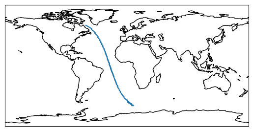
We can also, of course, consider physical variables along the section, such as total precipitation, averaged over time.
ds_section["tp"].sel(time="2020").mean("time").plot(x="lat")
[<matplotlib.lines.Line2D at 0x7f9db714e490>]
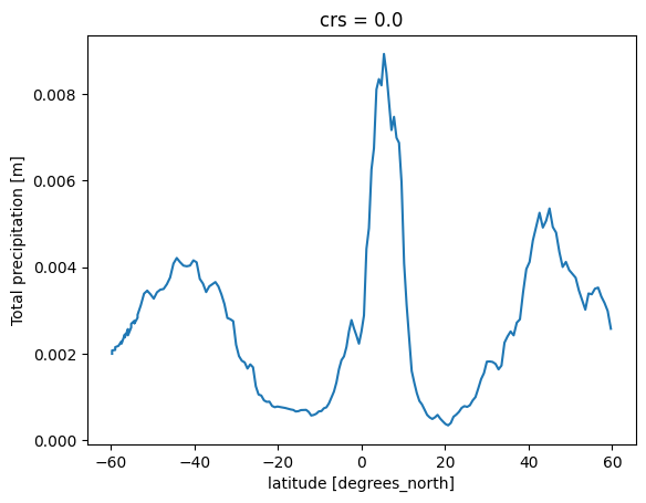
Scientific regions#
For some analysis, specifically defined “scientific regions” have been defined.
The regionmask package provides a convenient interface to apply these regions to latitude and longitude coordinates.
Our select_regionmask() function is a convenient wrapper that makes use of the region masks to select HEALPix maps.
By default, the AR6 climate reference regions (Iturbide et al. (2020)) are used.
Other defined regions provided by regionmask can be passed via the defined_regions keyword.
Regions can be selected by passing their number or abbreviation. Here, we select Central and South America:
import cartopy.feature as cf


ds_roi = egh.select_regionmask(ds, [9, 10, 11, 12, 13, 14, 15])

fig, ax = plt.subplots(subplot_kw={"projection": ccrs.PlateCarree()})
ax.add_feature(cf.COASTLINE, lw=0.8)
ax.add_feature(cf.BORDERS, lw=0.4)
ax.set_extent([-100, -20, -60, 20])
egh.healpix_show(ds_roi["2t"].sel(time="2020-02-01"))
<matplotlib.image.AxesImage at 0x7f9dabb00cd0>
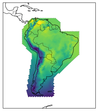
Again, we can also do arbitrary analysis on our selected data
ds_roi["2t"].mean("cell").plot()
[<matplotlib.lines.Line2D at 0x7f9dabb03ed0>]
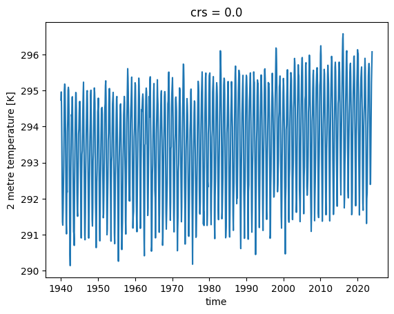
Countries#
A notable example of a different set of defined regions is countries as defined by Natural Earth. These regions can be used in exactly the same way as other defined regions:
import regionmask


ne_countries = regionmask.defined_regions.natural_earth_v5_1_2.countries_50
ds_brazil = egh.select_regionmask(ds, "Brazil", defined_regions=ne_countries)

fig, ax = plt.subplots(subplot_kw={"projection": ccrs.PlateCarree()})
ax.add_feature(cf.COASTLINE, lw=0.8)
ax.add_feature(cf.BORDERS, lw=0.4)
ax.set_extent([-100, -20, -60, 20])
egh.healpix_show(ds_brazil["2t"].sel(time="2020").mean("time"))
<matplotlib.image.AxesImage at 0x7f9da905c2d0>