
Calculating zonal means#
import intake
import matplotlib.pyplot as plt
import numpy as np
import xarray as xr
In this example we will compute the zonal-mean surface temperature of the ICON native grid.
cat = intake.open_catalog("https://data.nextgems-h2020.eu/online.yaml")
ds = cat.tutorial["ICON.native.2d_P1D_mean"](chunks={}).to_dask()
ds
<xarray.Dataset> Size: 844MB
Dimensions:             (time: 31, ncells: 1310720)
Coordinates:
  * time                (time) datetime64[ns] 248B 2020-01-01T23:59:59 ... 20...
    cell_sea_land_mask  (ncells) float64 10MB dask.array<chunksize=(1310720,), meta=np.ndarray>
    lat                 (ncells) float64 10MB dask.array<chunksize=(1310720,), meta=np.ndarray>
    lon                 (ncells) float64 10MB dask.array<chunksize=(1310720,), meta=np.ndarray>
Dimensions without coordinates: ncells
Data variables:
    hus2m               (time, ncells) float32 163MB dask.array<chunksize=(1, 1310720), meta=np.ndarray>
    psl                 (time, ncells) float32 163MB dask.array<chunksize=(1, 1310720), meta=np.ndarray>
    ts                  (time, ncells) float32 163MB dask.array<chunksize=(1, 1310720), meta=np.ndarray>
    uas                 (time, ncells) float32 163MB dask.array<chunksize=(1, 1310720), meta=np.ndarray>
vas (time, ncells) float32 163MB dask.array<chunksize=(1, 1310720), meta=np.ndarray>The general idea#
behind the zonal average is to calculate a weighted average of values in a certain latitude bin. Therefore, in a first step, we count how many cells are in given equidistant latitude bins.
hist_opts = dict(bins=128, range=(-90, 90))
cells_per_bin, lat_bins = np.histogram(ds.lat, **hist_opts)
Now comes the trick! In a next step, we will repeat the histogram but account a weight to each cell.
Usually, histogram will weight each data point with one, i.e. it will count the values in a certain bin.
Here, we will weight each data point with the surface temperature.
Thereby, we will compute the cumulative sum of all temperatures in a given latitude bin.
Tip
The np.histogram function is more efficient when passing a range and a number of bins.
This is because, when constructing the bins internally, the function can assume equidistant bin sizes.
This is not the case when passing a sequence of bins directly.
varsum_per_bin, _ = np.histogram(
    ds.lat, weights=ds.ts.isel(time=1), **hist_opts
)
The zonal mean can now be computed by dividing the cumulative values of the temperature with the number of cells in each bin.
zonal_mean = varsum_per_bin / cells_per_bin
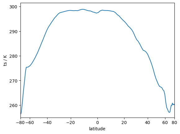
We can check our result by plotting the zonal mean as a function of the latitdue bins. While doing so, we will scale the bins by their area so that the visual appearance of each latitude bin represents their actual proportion.
fig, ax = plt.subplots()
ax.plot(0.5 * (lat_bins[1:] + lat_bins[:-1]), zonal_mean)
ax.set_ylabel("ts / K")
ax.set_ylim(bottom=255)

# Scale the x-axis to account for differences in area with latitude.
ax.set_xscale("function", functions=(lambda d: np.sin(np.deg2rad(d)), lambda d: np.arcsin(np.deg2rad(d))))
ax.set_xlim(-80, 80)
ax.set_xlabel("latitude")
Text(0.5, 0, 'latitude')
Note
The concept of using histograms to compute zonal means can also be generalized across other dimensions, i.e., a meridional mean or to compute distributions in temperature or humidity space.
Multi-dimensional input#
Until now, we used data at a single time step to illustrate the general idea of calculating zonal means by using histograms.
However, most real-world data has several other dimensions like time or height.
A straight-forward way to calculate zonal means for this kind of data is to unravel it, i.e., to get rid off every dimensions.
This approach, however, will loose all information of the thrown away axes; data at different heights or times will be mixed.
Fortunately, there are alternatives that allow us to calculate zonal means while maintaining the dimensional structure of our dataset.
We achieve this by using xr.apply_ufunc which lifts a function (in this case _compute_varsum) from (numpy) arrays to (xarray) DataArrays.
This lifting into the world of DataArrays involves describing the dimensions, shapes and data types which the function cares about. Afterwards, xarray applies the usual looping and broadcasting rules over the dimensions the functions does not care about. Any necessary looping may then be carried out in parallel (e.g. using dask).
def calc_zonal_mean(variable, **hist_opts):
    """Compute a zonal-mean (along `clat`) for multi-dimensional input."""
    counts_per_bin, bin_edges = np.histogram(variable.lat, **hist_opts)

    def _compute_varsum(var, **kwargs):
        """Helper function to compute histogram for a single timestep."""
        varsum_per_bin, _ = np.histogram(variable.lat, weights=var, **kwargs)
        return varsum_per_bin

    # For more information see:
    # https://docs.xarray.dev/en/stable/generated/xarray.apply_ufunc.html
    varsum = xr.apply_ufunc(
        _compute_varsum,  # function to map
        variable,  # variables to loop over
        kwargs=hist_opts,  # keyword arguments passed to the function
        input_core_dims=[["ncells"]],  # dimensions that should not be kept
        # Description of the output dataset
        dask="parallelized",
        vectorize=True,
        output_core_dims=[("lat_bins",)],
        dask_gufunc_kwargs={
            "output_sizes": {"lat_bins": hist_opts["bins"]},
        },
        output_dtypes=["f8"],
    )

    return varsum / counts_per_bin, bin_edges
Using this function we can calculate the zonal means along the time dimension.
zonal_means, lat_bins = calc_zonal_mean(ds.ts, **hist_opts)
zonal_means
<xarray.DataArray 'ts' (time: 31, lat_bins: 128)> Size: 32kB
dask.array<truediv, shape=(31, 128), dtype=float64, chunksize=(1, 128), chunktype=numpy.ndarray>
Coordinates:
  * time     (time) datetime64[ns] 248B 2020-01-01T23:59:59 ... 2020-01-31T23...
Dimensions without coordinates: lat_bins
Attributes:
    CDI_grid_type:                unstructured
    long_name:                    surface temperature
    number_of_grid_in_reference:  1
    param:                        0.0.0
    standard_name:                surface_temperature
units: KWe can now either plot the zonal means for individual timesteps or the whole dataset.
Warning
The function xr.apply_ufunc() returns a lazy data array, meaning that the data is only loaded when requested.
Computing a histogram for the entire time period thus requires loading all the data.
fig, ax = plt.subplots()

ax.plot(0.5 * (lat_bins[1:] + lat_bins[:-1]), zonal_means.isel(time=1))
ax.set_ylabel("ts / K")
ax.set_ylim(bottom=255)

# Scale the x-axis to account for differences in area with latitude.
ax.set_xscale("function", functions=(lambda d: np.sin(np.deg2rad(d)), lambda d: np.arcsin(np.deg2rad(d))))
ax.set_xlim(-80, 80)
ax.set_xlabel("latitude")
Text(0.5, 0, 'latitude')