
Vertical interpolation on non-coordinate dimensions#
Vertical interpolation is a very common task in geoscientific data analysis: model output is often defined on terrain-following or hybrid vertical coordinates, while analysis and diagnostics are typically performed on fixed pressure or height levels.
In simple cases, vertical interpolation can be done using xarray.interp().
However, this requires the vertical coordinate to be a 1D coordinate variable.
In many real-world datasets, the vertical coordinate itself varies with time and horizontal position.
In that case, it is no longer a true coordinate from xarray’s perspective, and a different approach is required.
This notebook demonstrates how to perform vectorized vertical interpolation with xarray when the vertical coordinate depends on multiple dimensions.
Opening the dataset#
First, we open a global ICON dataset stored on the native horizontal and vertical grids.
For performance reasons, we explicitly chunk the dataset so that entire vertical columns are kept in one Dask chunk.
This is important because interpolation will operate along the vertical dimension.
import intake


cat = intake.open_catalog("https://data.nextgems-h2020.eu/online.yaml")
ds = cat.tutorial["ICON.native.3d_P1D_mean"](chunks={"height": -1}).to_dask()
ds
<xarray.Dataset> Size: 4GB
Dimensions:             (time: 4, height: 45, ncells: 1310720)
Coordinates:
  * time                (time) datetime64[ns] 32B 2026-01-02 ... 2026-01-05
  * height              (height) float64 360B 1.0 3.0 5.0 7.0 ... 85.0 87.0 89.0
    cell_sea_land_mask  (ncells) float64 10MB dask.array<chunksize=(1310720,), meta=np.ndarray>
    lat                 (ncells) float64 10MB dask.array<chunksize=(1310720,), meta=np.ndarray>
    lon                 (ncells) float64 10MB dask.array<chunksize=(1310720,), meta=np.ndarray>
Dimensions without coordinates: ncells
Data variables:
    pfull               (time, height, ncells) float32 944MB dask.array<chunksize=(1, 45, 1310720), meta=np.ndarray>
    ta                  (time, height, ncells) float32 944MB dask.array<chunksize=(1, 45, 1310720), meta=np.ndarray>
    ua                  (time, height, ncells) float32 944MB dask.array<chunksize=(1, 45, 1310720), meta=np.ndarray>
va (time, height, ncells) float32 944MB dask.array<chunksize=(1, 45, 1310720), meta=np.ndarray>Why interp() is not sufficient here#
The variables we want to interpolate (e.g. temperature and wind components) have dimensions:
ds.ta.dims
('time', 'height', 'ncells')
The atmospheric pressure (pfull) also varies along time, height, and ncells. This means:
pfullis not a 1D coordinatexarray.interp()cannot be used directly
Conceptually, what we want is:
For every
(time, ncells)column, interpolate the vertical profile independently.
To do this efficiently and in a Dask-compatible way, we use xarray.apply_ufunc().
Defining a 1D interpolation kernel#
We first define a small NumPy-based helper function that interpolates one vertical profile onto new target levels.
This function operates purely on NumPy arrays and knows nothing about xarray or Dask.
xarray.apply_ufunc() will take care of vectorizing it over the remaining dimensions.
import numpy as np


def interp_1d(y, x, x_new):
    return np.interp(x_new, x, y, left=np.nan, right=np.nan)
Target pressure levels#
Next, we define the pressure levels onto which we want to interpolate the data. These levels are fixed and shared across all columns.
p_levels = 100 * np.array(
    [
        1000, 975, 950, 925, 900, 875, 850, 800, 750, 700, 600,
        500, 400, 300, 250, 200, 150, 100, 70, 50, 30, 20, 10, 5, 1
    ]
)
Vectorized vertical interpolation with apply_ufunc()#
We now apply the interpolation function to the dataset.
Key points to note:
input_core_dimsspecifies that interpolation happens alongheightvectorize=Trueapplies the function independently overtimeandncellsdask="parallelized"enables lazy, parallel executionWe lazily interpolate the whole dataset in one call
import xarray as xr


ds_plev = xr.apply_ufunc(
    interp_1d,
    ds,
    ds.pfull,
    p_levels,
    input_core_dims=[["height"], ["height"], ["plev"]],
    output_core_dims=[["plev"]],
    vectorize=True,
    dask="parallelized",
).assign_coords(plev=p_levels)

ds_plev
<xarray.Dataset> Size: 4GB
Dimensions:             (time: 4, ncells: 1310720, plev: 25)
Coordinates:
  * time                (time) datetime64[ns] 32B 2026-01-02 ... 2026-01-05
  * plev                (plev) int64 200B 100000 97500 95000 ... 1000 500 100
    cell_sea_land_mask  (ncells) float64 10MB dask.array<chunksize=(1310720,), meta=np.ndarray>
    lat                 (ncells) float64 10MB dask.array<chunksize=(1310720,), meta=np.ndarray>
    lon                 (ncells) float64 10MB dask.array<chunksize=(1310720,), meta=np.ndarray>
Dimensions without coordinates: ncells
Data variables:
    pfull               (time, ncells, plev) float64 1GB dask.array<chunksize=(1, 1310720, 25), meta=np.ndarray>
    ta                  (time, ncells, plev) float64 1GB dask.array<chunksize=(1, 1310720, 25), meta=np.ndarray>
    ua                  (time, ncells, plev) float64 1GB dask.array<chunksize=(1, 1310720, 25), meta=np.ndarray>
va (time, ncells, plev) float64 1GB dask.array<chunksize=(1, 1310720, 25), meta=np.ndarray>Memory footprint
Vertical interpolation requires loading entire vertical columns at once. If the data is also stored in large horizontal chunks (for example, full global fields), this can result in very high memory usage.
Inspecting the result#
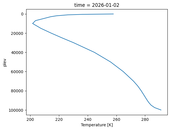
As a quick sanity check, we plot the globally averaged temperature profile for a single time slice.
ds_plev.ta.sel(time="2026-01-02").mean("ncells").plot(y="plev", yincrease=False)
[<matplotlib.lines.Line2D at 0x7f5a60532490>]
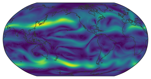
Finally, we compute wind speed from the wind components and visualize it at 500 hPa.
from easygems.resample import KDTreeResampler
from easygems.show import map_show


ds_plev = ds_plev.assign(wind=lambda dx: np.hypot(dx.ua, dx.va))

kd_resampler = KDTreeResampler(lat=ds_plev.lat, lon=ds_plev.lon)
map_show(ds_plev.wind.sel(time="2026-01-02", plev=200e2).values, kd_resampler)
<matplotlib.image.AxesImage at 0x7f5a5bcfd940>
Takeaway#
When a “coordinate” varies along the same dimension it indexes, it must be treated as data, not as an xarray coordinate.
In these situations, xr.apply_ufunc() provides a powerful and scalable way to express column-wise operations such as vertical interpolation—without explicit Python loops and fully compatible with Dask.