Plotting geospatial data on a map#
Plotting in pixel-space#
When working with geospatial data, it is common to remap datasets before plotting them on a map. While this approach is convenient, it not only obscures where the data actually originates on Earth but also requires substantial computational resources, especially for high-resolution fields. Moreover, this workflow performs an often overlooked extra step: even after remapping to a new grid, the data is again resampled into pixel-space during plotting. In other words, traditional approaches effectively remap the data twice.
In this tutorial, we take a different route: we work directly in pixel-space. Instead of remapping the data upfront, we first create a Cartopy GeoAxes and then determine the geographic coordinates associated with each pixel on that axis. By sampling our original dataset at those coordinates, we construct the map directly from the source data. This method avoids unnecessary interpolation, reduces overhead, and provides a clearer view of how data and map projections interact.
HEALPix resampling#
As a first example, we will plot data on the HEALPix grid. For this purpose, we will use a HEALPix-ified version of the ERA5 reanalysis dataset.
import intake


cat = intake.open_catalog("https://data.nextgems-h2020.eu/online.yaml")
era5 = cat.ERA5(zoom=7).to_dask()
One of the defining properties of HEALPix is that the grid points closest to a given latitude and longitude can be queried efficiently based on analytical equations.
All that is required is knowledge of the defining parameters of the HEALPix grid, i.e. its refinement level and nesting scheme.
The easygems package provides a HEALPixResampler helper class that can be initialised using these parameters:
from easygems.healpix import get_nside
from easygems.resample import HEALPixResampler

hp_resampler = HEALPixResampler(nside=get_nside(era5))
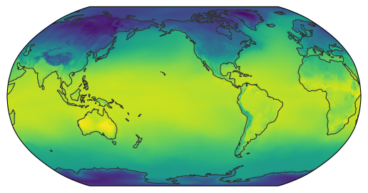
We can now pass both our dataset and the resampler to the map_show() function.
By default, map_show() creates a world map.
For each pixel, it internally determines the corresponding latitude and longitude, then uses the resampler to fill that pixel with the appropriate data value:
from easygems.show import map_show

map_show(era5["2t"].isel(time=0), resampler=hp_resampler);
Note
The resolution of the plot depends on the dots per inch (DPI) of the figure itself.
You can either pass the dpi keyword to map_show() or create your own Cartopy GeoAxes with an arbitrary DPI.
The resampler is designed to simply return values for a given coordinate. Therefore, it can also be used to create different types of map, such as contour lines:
from easygems.show import map_contour

map_contour(era5["2t"].isel(time=0), resampler=hp_resampler);
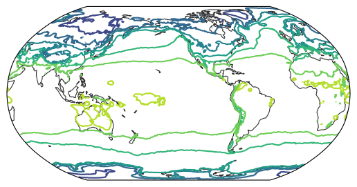
Tip
Both map_show() and map_contour() can be used with any resampler.
For smooth contour lines, it is recommended to use an interpolating resampler (see, e.g., Delaunay triangulation).
Nearest-neighbor resampling#
Next, we will load an ICON dataset on its native grid. The ICON grid is based on an icosahedron that is bisected to create different resolutions, which are then further processed for the numerical stability of simulations. While visually still close to the original icosahedron, the resulting grid points are technically a rather unstructured set of latitudes and longitudes.
import xarray as xr

from easygems.show import map_show


cat = intake.open_catalog("https://data.nextgems-h2020.eu/online.yaml")
icon = cat.tutorial["ICON.native.2d_PT6H_inst"](chunks={}).to_dask()
In order to resample the grid, we will construct a k-d tree to efficiently query nearest-neighbor points.
This querying is best done in xyz space to find the actual closest points at the poles and date line.
The easygems package does provide a convenience class for this:
from easygems.resample import KDTreeResampler

kd_resampler = KDTreeResampler(lat=icon.lat, lon=icon.lon)
Important
All resamplers must receive latitude and longitude in units of degrees.
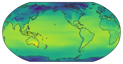
Again, we pass both our dataset and the resampler to the map_show() function:
map_show(icon["ts"].isel(time=-1), resampler=kd_resampler);
Delaunay triangulation#
Finally, there is a specialised resampler for plotting smoothed maps. It will perform a Delaunay triangulation and return a weighted average of the surrounding grid points. This can be particularly useful for smoothing contour lines or when creating plots on custom regional-scale maps:
import cartopy.crs as ccrs
import matplotlib.pyplot as plt
from easygems.resample import DelaunayResampler
tri_resampler = DelaunayResampler(lat=icon.lat, lon=icon.lon)
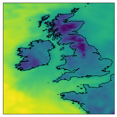
fig, ax = plt.subplots(subplot_kw={"projection": ccrs.PlateCarree()})
ax.set_extent([-12, 2, 46, 60])
ax.coastlines()
map_show(icon["ts"].isel(time=-1), resampler=tri_resampler, ax=ax);
Note
When creating a custom GeoAxes, it is important to explicitly set an extent using the .set_extent() or .set_global() methods.
This is because Cartopy creates maps with a minimal spatial extent by default, which leads to strange plotting artefacts.
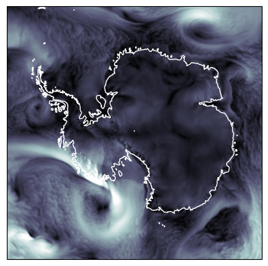
The poles and the Date Line#
When plotting geospatial data, wrapping coordinates around the North and South Poles or the International Date Line can cause issues. However, all resamplers are implemented in ways to account for the topology of spherical grids. Therefore, the plotting functions can be used with any Cartopy projection:
import numpy as np


icon = icon.assign(sfcwind=lambda dx: np.hypot(dx.uas, dx.vas))

fig, ax = plt.subplots(subplot_kw={'projection': ccrs.SouthPolarStereo()})
ax.set_extent([-180, 180, -90, -60], ccrs.PlateCarree())
ax.coastlines(color="white")
map_show(icon["sfcwind"].isel(time=-1), resampler=tri_resampler, vmax=30, cmap="bone", ax=ax);
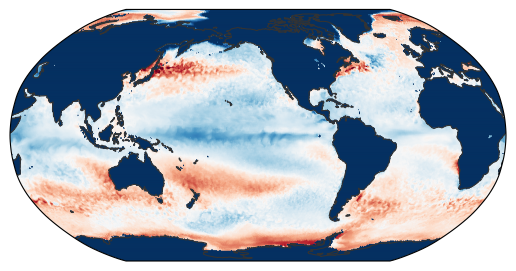
Plotting differences#
The idea of plotting in pixel-space can also be used to plot the difference between two fields on arbitrary grids. Because the two datasets live on different grids, each needs its own resampler to project onto a common pixel-space.
We can use the map_diff() function to plot the difference between two datasets directly.
The function signature is similar to map_show() but takes two data fields and their respective resamplers as input:
from easygems.show import map_diff

icon_ts = icon["ts"].sel(time="2020-01").mean("time")
era5_sst = era5["sst"].sel(time="2020-01").mean("time")

map_diff(
    icon_ts,
    kd_resampler,
    era5_sst,
    hp_resampler,
    cmap="RdBu_r",
    vmin=-10,
    vmax=10,
)
<matplotlib.image.AxesImage at 0x7f90f3f39d10>
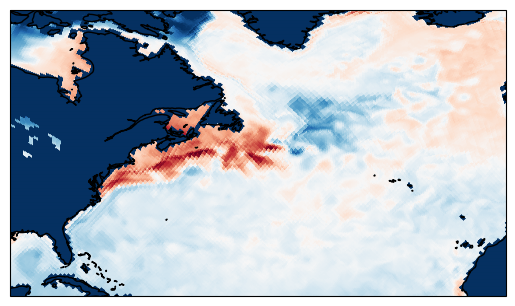
Just like the other plotting functions, one can also create a custom GeoAxes to plot on. Here we zoom into the North Atlantic to better inspect regional differences:
fig, ax = plt.subplots(subplot_kw={"projection": ccrs.PlateCarree()})
ax.set_extent([-90, -10, 20, 60])
ax.coastlines()
map_diff(
    icon_ts,
    kd_resampler,
    era5_sst,
    hp_resampler,
    cmap="RdBu_r",
    vmin=-10,
    vmax=10,
    ax=ax,
)
<matplotlib.image.AxesImage at 0x7f911859d090>